こちらの資料がソース。 rstudio-pubs-static.s3.amazonaws.com https://dss.princeton.edu/training/Panel101R.pdf
plmパッケージ
rdrr.io https://cran.r-project.org/web/packages/plm/plm.pdf
データの読み込み
library(foreign)
Panel <- read.dta("http://dss.princeton.edu/training/Panel101.dta")
データ
head(Panel)
  country year           y y_bin        x1         x2          x3   opinion op
1       A 1990  1342787840     1 0.2779036 -1.1079559  0.28255358 Str agree  1
2       A 1991 -1899660544     0 0.3206847 -0.9487200  0.49253848     Disag  0
3       A 1992   -11234363     0 0.3634657 -0.7894840  0.70252335     Disag  0
4       A 1993  2645775360     1 0.2461440 -0.8855330 -0.09439092     Disag  0
5       A 1994  3008334848     1 0.4246230 -0.7297683  0.94613063     Disag  0
6       A 1995  3229574144     1 0.4772141 -0.7232460  1.02968037 Str agree  1
プロット
変数yに関してのプロット。
coplot(y ~ year|country, type="l", data=Panel)    # Lines
coplot(y ~ year|country, type="b", data=Panel)  # Points and lines


散布図。
library(car)
scatterplot(y~year|country, boxplots=FALSE, smooth=TRUE, reg.line=FALSE, data=Panel)

固定効果モデル
共分散モデル、Within推定量、個体ダミー変数モデル、最小二乗ダミー変数モデル
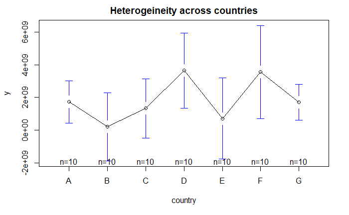
yと国に関しての描画。
library(gplots)
plotmeans(y ~ country, main="Heterogeineity across countries", data=Panel)
plotmeansは、平均値の95%信頼区間を描画する。
library(gplots)
plotmeans(y ~ year, main="Heterogeineity across countries", data=Panel)

回帰分析
ols <-lm(y ~ x1, data=Panel)
summary(ols)
Coefficients:
             Estimate Std. Error t value Pr(>|t|)
(Intercept) 1.524e+09  6.211e+08   2.454   0.0167 *
x1          4.950e+08  7.789e+08   0.636   0.5272
作図
yhat <- ols$fitted
plot(Panel$x1, Panel$y, pch=19, xlab="x1", ylab="y")
abline(lm(Panel$y~Panel$x1),lwd=3, col="red")

ggplotの場合。
library(ggplot2)
ggplot(Panel, aes(x = x1, y = y))+
  geom_point() +
  geom_smooth(method=lm)

重回帰分析・国を追加
fixed.dum <-lm(y ~ x1 + factor(country) - 1, data=Panel)
summary(fixed.dum)
Coefficients:
                   Estimate Std. Error t value Pr(>|t|)
x1                2.476e+09  1.107e+09   2.237  0.02889 *
factor(country)A  8.805e+08  9.618e+08   0.916  0.36347
factor(country)B -1.058e+09  1.051e+09  -1.006  0.31811
factor(country)C -1.723e+09  1.632e+09  -1.056  0.29508
factor(country)D  3.163e+09  9.095e+08   3.478  0.00093 ***
factor(country)E -6.026e+08  1.064e+09  -0.566  0.57329
factor(country)F  2.011e+09  1.123e+09   1.791  0.07821 .
factor(country)G -9.847e+08  1.493e+09  -0.660  0.51190
yhat <- fixed.dum$fitted
library(car)
scatterplot(yhat~Panel$x1|Panel$country, boxplots=FALSE, xlab="x1", ylab="yhat",smooth=FALSE)
abline(lm(Panel$y~Panel$x1),lwd=3, col="red")

要因変数(国)の各要素は、各国特有の効果を吸収している。予測変数x1はOLSモデルでは有意ではなかったが、一旦国ごとの差異をコントロールすると、OLS_DUM(すなわちLSDVモデル)でx1は有意となる。
固定効果:n 個のエンティティ固有の切片(plmパッケージを使用)
y: 従属変数
x1: 独立変数
data: データ
index: パネルセッティング
model="within": 固定効果オプション
library(plm)
fixed <- plm(y ~ x1, data=Panel, index=c("country", "year"), model="within")
summary(fixed)
結果。
Balanced Panel: n = 7, T = 10, N = 70

Residuals:
     Min.   1st Qu.    Median      Mean   3rd Qu.      Max.
-8.63e+09 -9.70e+08  5.40e+08  0.00e+00  1.39e+09  5.61e+09

Coefficients:
     Estimate Std. Error t-value Pr(>|t|)
x1 2475617827 1106675594   2.237  0.02889 *
---
Signif. codes:  0 ‘***’ 0.001 ‘**’ 0.01 ‘*’ 0.05 ‘.’ 0.1 ‘ ’ 1

Total Sum of Squares:    5.2364e+20
Residual Sum of Squares: 4.8454e+20
R-Squared:      0.074684
Adj. R-Squared: -0.029788
F-statistic: 5.00411 on 1 and 62 DF, p-value: 0.028892
n = グループ/パネル数
T = 年
N = 総観測数
Coefficients:Estimate
x1の係数は、Xが1単位増加したときに、Yが国ごとに平均してどれだけ時間的に変化するかを示している。
x Pr(>|t|):0.02889:
Pr(>|t|)= 両側p値は,各係数が0と異なるという仮説を検定する。これを棄却するには,p値が0.05 (95%, 0.10のアルファも選択できる)でなければならず、これが事実であれば、その変数が従属変数(y)に有意な影響を持つことができる。
p-value: 0.028892:
この数値が< 0.05であればこのモデルは問題ない。これは、モデルのすべての係数が0に比べて異なるかどうかを見る検定(F)である。
fixef(fixed) # 固定効果(各国の定数)を表示する
結果。
          A           B           C           D           E           F           G
  880542404 -1057858363 -1722810755  3162826897  -602622000  2010731793  -984717493
pFtest(fixed, ols) # 固定効果に対する検定。固定効果よりもOLSの方が良いのか?
結果。
data:  y ~ x1
F = 2.9655, df1 = 6, df2 = 62, p-value = 0.01307
alternative hypothesis: significant effects
p値が0.05未満であれば、固定効果モデルがより良い選択となる。
ランダム効果モデル (ランダム切片, 部分プーリングモデル)
model="random"と指定する。
random <- plm(y ~ x1, data=Panel, index=c("country", "year"), model="random")
summary(random)
結果。
Balanced Panel: n = 7, T = 10, N = 70

Effects:
                    var   std.dev share
idiosyncratic 7.815e+18 2.796e+09 0.873
individual    1.133e+18 1.065e+09 0.127
theta: 0.3611

Residuals:
     Min.   1st Qu.    Median      Mean   3rd Qu.      Max.
-8.94e+09 -1.51e+09  2.82e+08  0.00e+00  1.56e+09  6.63e+09

Coefficients:
              Estimate Std. Error z-value Pr(>|z|)
(Intercept) 1037014284  790626206  1.3116   0.1896
x1          1247001782  902145601  1.3823   0.1669

Total Sum of Squares:    5.6595e+20
Residual Sum of Squares: 5.5048e+20
R-Squared:      0.02733
Adj. R-Squared: 0.013026
Chisq: 1.91065 on 1 DF, p-value: 0.16689
係数の解釈は難しい。なぜなら、係数はwithin効果とbetween果の両方を含んでいるからである。TSCSの場合、Xが時間軸で1単位、国別で1単位変化したときのXのYに対する平均的な効果を表している。
Pr(>|t|)= 両側検定のp値は,各係数が0と異なるという仮説を検定する。これを棄却するには,p値が0.05 (95%, 0.10のアルファも選択できる)でなければならず,これが事実であれば,その変数が従属変数(y)に有意な影響を持つことができる.
カイ二乗検定のP値:この数値が<0.05であれば、そのモデルはOKである。これは、モデル中のすべての係数がゼロと異なるかどうかを確認する検定 (F)である。
パネルデータとして設定(上記のモデルを実行する別の方法)
Panel.set <- pdata.frame(Panel, index = c("country", "year"))
plmパッケージでは、plm.data()はpdata.frame()に変更されている。
パネル設定によるランダム効果 (上記と同じ出力)
random.set <- plm(y ~ x1, data = Panel.set, model="random")
summary(random.set)
結果。
Balanced Panel: n = 7, T = 10, N = 70

Effects:
                    var   std.dev share
idiosyncratic 7.815e+18 2.796e+09 0.873
individual    1.133e+18 1.065e+09 0.127
theta: 0.3611

Residuals:
     Min.   1st Qu.    Median      Mean   3rd Qu.      Max.
-8.94e+09 -1.51e+09  2.82e+08  0.00e+00  1.56e+09  6.63e+09

Coefficients:
              Estimate Std. Error z-value Pr(>|z|)
(Intercept) 1037014284  790626206  1.3116   0.1896
x1          1247001782  902145601  1.3823   0.1669

Total Sum of Squares:    5.6595e+20
Residual Sum of Squares: 5.5048e+20
R-Squared:      0.02733
Adj. R-Squared: 0.013026
Chisq: 1.91065 on 1 DF, p-value: 0.16689
固定効果がランダム効果か?
固定効果かランダム効果かを決定するために、帰無仮説は、望ましいモデルがランダム効果で、代替モデルが固定効果であるとするHausman検定を実行できる(Green, 2008, chapter 9を参照)。 これは基本的に、固有誤差(ui)が回帰変数と相関しているかどうかを検定するもので、帰無仮説は相関していないというものである。
固定効果モデルを実行して推定値を保存し、次にランダム・モデルを実行して推定値を保存し、そして検定を実行する。P値が有意であれば(たとえば、<0.05)、固定効果を使用し、そうでなければランダム効果を使用する。
phtest(fixed, random)
結果。
 Hausman Test

data:  y ~ x1
chisq = 3.674, df = 1, p-value = 0.05527
alternative hypothesis: one model is inconsistent
p-valueの数値が0.05未満であれば、固定効果を用いる。
その他のテスト・測定項目
時間固定効果に対する検定
fixed <- plm(y ~ x1, data=Panel, index=c("country", "year"), model="within")
fixed.time <- plm(y ~ x1 + factor(year), data=Panel, index=c("country", "year"), model="within")
summary(fixed.time)
結果。
Coefficients:
                   Estimate Std. Error t-value Pr(>|t|)
x1               1389050354 1319849567  1.0524  0.29738
factor(year)1991  296381559 1503368528  0.1971  0.84447
factor(year)1992  145369666 1547226548  0.0940  0.92550
factor(year)1993 2874386795 1503862554  1.9113  0.06138 .
factor(year)1994 2848156288 1661498927  1.7142  0.09233 .
factor(year)1995  973941306 1567245748  0.6214  0.53698
factor(year)1996 1672812557 1631539254  1.0253  0.30988
factor(year)1997 2991770063 1627062032  1.8388  0.07156 .
factor(year)1998  367463593 1587924445  0.2314  0.81789
factor(year)1999 1258751933 1512397632  0.8323  0.40898
---
Signif. codes:  0 ‘***’ 0.001 ‘**’ 0.01 ‘*’ 0.05 ‘.’ 0.1 ‘ ’ 1

Total Sum of Squares:    5.2364e+20
Residual Sum of Squares: 4.0201e+20
R-Squared:      0.23229
Adj. R-Squared: 0.00052851
F-statistic: 1.60365 on 10 and 53 DF, p-value: 0.13113
個体効果および時間効果に関するF検定 F Test for Individual and/or Time Effects
withinモデルとpoolingモデルの比較に基づく個人効果および時間効果の検定。
pFtest(fixed.time, fixed)
結果。
 F test for individual effects

data:  y ~ x1 + factor(year)
F = 1.209, df1 = 9, df2 = 53, p-value = 0.3094
alternative hypothesis: significant effects
この数値が<0.05であれば 時間固定効果を用いる。この例では、時間固定効果を使用する必要はない。
パネルモデルに対するラグランジュFF乗数検定 Lagrange FF Multiplier Tests for Panel Models
パネルモデルにおける個人効果および時間効果の検定である。
plmtest(fixed, c("time"), type=("bp"))
 Lagrange Multiplier Test - time effects (Breusch-Pagan) for balanced panels

data:  y ~ x1
chisq = 0.16532, df = 1, p-value = 0.6843
alternative hypothesis: significant effects
この数値が<0.05であれば 時間固定効果を用いる。この例では、時間固定効果を使用する必要はない。
ランダム効果に対する検定 Breusch-Pagan ラグランジュ乗数(LM)
pool <- plm(y ~ x1, data=Panel, index=c("country", "year"), model="pooling")
summary(pool)
結果。
Residuals:
     Min.   1st Qu.    Median      Mean   3rd Qu.      Max.
-9.55e+09 -1.58e+09  1.55e+08  0.00e+00  1.42e+09  7.18e+09

Coefficients:
              Estimate Std. Error t-value Pr(>|t|)
(Intercept) 1524319070  621072624  2.4543  0.01668 *
x1           494988914  778861261  0.6355  0.52722
---
Signif. codes:  0 ‘***’ 0.001 ‘**’ 0.01 ‘*’ 0.05 ‘.’ 0.1 ‘ ’ 1

Total Sum of Squares:    6.2729e+20
Residual Sum of Squares: 6.2359e+20
R-Squared:      0.0059046
Adj. R-Squared: -0.0087145
F-statistic: 0.403897 on 1 and 68 DF, p-value: 0.52722
LM検定は,ランダム効果回帰と単純なOLS回帰のどちらかを決定するのに役立つ。
LM検定での帰無仮説は,実体間の分散が0であるということである。これは,単位間の有意な差がない(すなわち,パネル効果がない)ことを意味する。
plmtest(pool, type=c("bp"))
 Lagrange Multiplier Test - (Breusch-Pagan) for balanced panels

data:  y ~ x1
chisq = 2.6692, df = 1, p-value = 0.1023
alternative hypothesis: significant effects
ここでは、帰無値を棄却できず、ランダム効果が適切でないと結論づけられた。これは、国による有意差の証拠がない 国による有意差の証拠がないため、単純なOLS回帰を実行することができる。
Breusch-Pagan LMの独立性検定とPasaran CD検定による横断的依存性/同時発生的相関の検定
Baltagiによれば,クロスセクション依存性 cross-sectional dependence は,長い時系列を持つマクロパネルでは問題である。これは,ミクロ・パネル(数年,多数のケース)では,あまり問題にならない.
独立性のB-P/LM検定とPasaran CD検定における帰無仮説は,主体間の残差は相関しないことである。 B-P/LMおよびPasaran CD(断面依存性)検定は,残差がエンティティ間*で相関しているかどうかを検定するために使用される.クロスセクション依存性は,検定結果にバイアスをもたらす可能性がある(同時計数相関 contemporaneous correlation ともいう)。
*Source: Hoechle, Daniel, “Robust Standard Errors for Panel Regressions with Cross-Sectional Dependence”, http://fmwww.bc.edu/repec/bocode/x/xtscc_paper.pdf
fixed <- plm(y ~ x1, data=Panel, index=c("country", "year"), model="within")
pcdtest(fixed, test = c("lm"))
結果。
 Breusch-Pagan LM test for cross-sectional dependence in panels

data:  y ~ x1
chisq = 28.914, df = 21, p-value = 0.1161
alternative hypothesis: cross-sectional dependence
pcdtest(fixed, test = c("cd"))
 Pesaran CD test for cross-sectional dependence in panels

data:  y ~ x1
z = 1.1554, p-value = 0.2479
alternative hypothesis: cross-sectional dependence
系列相関の検定
系列相関検定は,長い時系列を持つマクロパネルに適用される。ミクロ・パネル(年数が非常に少ない)では問題ない。帰無仮説は,系列相関がないことである.
pbgtest(fixed)
結果。
 Breusch-Godfrey/Wooldridge test for serial correlation in panel models

data:  y ~ x1
chisq = 14.137, df = 10, p-value = 0.1668
alternative hypothesis: serial correlation in idiosyncratic errors
p-value=0.1668なので、系列相関がない。
単位根/定常性の検定
確率的トレンドを確認するためのDickey-Fuller検定。帰無仮説は、系列が単位根を持つ(すなわち、非定常)ことである。単位根が存在する場合、変数の第1階差を取ることができる。
Panel.set <- plm.data(Panel, index = c("country", "year"))
library(tseries)
adf.test(Panel.set$y, k=2)
結果。
 Augmented Dickey-Fuller Test

data:  Panel.set$y
Dickey-Fuller = -3.9051, Lag order = 2, p-value = 0.0191
alternative hypothesis: stationary
p値<0.05の場合、単位根は存在しない。
分散不均一性 heteroskedasticity の検定
library(lmtest)
bptest(y ~ x1 + factor(country), data = Panel, studentize=F)
 Breusch-Pagan test

data:  y ~ x1 + factor(country)
BP = 14.606, df = 7, p-value = 0.04139
P<0.05であるため分散不均一性 heteroskedasticityが検出された。
分散不均一性が検出された場合、ロバスト共分散行列を使用してそれを考慮することができる。
分散不均一性を制御--ロバスト共分散行列推定法(Sandwich推定法)
vcovHC-関数は、3つの異種分散共分散推定量を推定します。
- "white1" - 一般的な異種分散性を持つが系列相関を持たない場合。ランダム効果に推奨。
- "white2" - "white1 "をグループ内の共通分散に制限したもの。ランダム効果に推奨
- "arellano" - 分散不均一性と系列相関の両方。固定効果に推奨。
以下のオプションが適用される*。
- HC0 - 分散不均一性の整合性。デフォルト。
- HC1,HC2,HC3 - サンプル数が少ない場合に推奨される。HC3は、影響力のあるオブザベーションにあまりきを置かない.
- HC4 - 影響力のあるオブザベーションを持つ小さな標本.
- HAC - 分散不均一性と自己相関の整合性(詳細は, ?vcovHAC とタイプ).
*Kleiber and Zeileis, 2008.
分散不均一性の制御 ランダム効果
random <- plm(y ~ x1, data=Panel, index=c("country", "year"), model="random")
coeftest(random) # 本来の係数 Original coefficients
結果。
t test of coefficients:

              Estimate Std. Error t value Pr(>|t|)
(Intercept) 1037014284  790626206  1.3116   0.1941
x1          1247001782  902145601  1.3823   0.1714
coeftest(random, vcovHC) # 分散不均一性整合係数 Heteroskedasticity consistent coefficients
結果。
t test of coefficients:

              Estimate Std. Error t value Pr(>|t|)
(Intercept) 1037014284  907983029  1.1421   0.2574
x1          1247001782  828970247  1.5043   0.1371
# 分散不均一性整合係数タイプ 3Heteroskedasticity consistent coefficients, type 3
coeftest(random, vcovHC(random, type = "HC3"))
結果。
t test of coefficients:

              Estimate Std. Error t value Pr(>|t|)
(Intercept) 1037014284  943438284  1.0992   0.2756
x1          1247001782  867137585  1.4381   0.1550
係数のHC標準誤差を以下に示す
t(sapply(c("HC0", "HC1", "HC2", "HC3", "HC4"), function(x) sqrt(diag(vcovHC(random, type = x)))))
    (Intercept)        x1
HC0   907983029 828970247
HC1   921238957 841072643
HC2   925403820 847733474
HC3   943438284 867137584
HC4   941376033 866024033
標準誤差は、HCの種類によって異なる。
分散不均一性の制御・固定効果
fixed <- plm(y ~ x1, data=Panel, index=c("country", "year"), model="within")
coeftest(fixed) # 本来の係数Original coefficients
結果。
t test of coefficients:

     Estimate Std. Error t value Pr(>|t|)
x1 2475617827 1106675594   2.237  0.02889 *
---
Signif. codes:  0 ‘***’ 0.001 ‘**’ 0.01 ‘*’ 0.05 ‘.’ 0.1 ‘ ’ 1
coeftest(fixed, vcovHC) # 分散不均一性整合係数 Heteroskedasticity consistent coefficients
結果。
t test of coefficients:

     Estimate Std. Error t value Pr(>|t|)
x1 2475617827 1358388942  1.8225  0.07321 .
---
Signif. codes:  0 ‘***’ 0.001 ‘**’ 0.01 ‘*’ 0.05 ‘.’ 0.1 ‘ ’ 1
# 分散不均一性整合係数 (Arellano)
coeftest(fixed, vcovHC(fixed, method = "arellano"))
結果。
t test of coefficients:

     Estimate Std. Error t value Pr(>|t|)
x1 2475617827 1358388942  1.8225  0.07321 .
---
Signif. codes:  0 ‘***’ 0.001 ‘**’ 0.01 ‘*’ 0.05 ‘.’ 0.1 ‘ ’ 1
# 分散不均一性整合係数タイプ 3Heteroskedasticity consistent coefficients, type 3
coeftest(fixed, vcovHC(fixed, type = "HC3"))
結果。
t test of coefficients:

     Estimate Std. Error t value Pr(>|t|)
x1 2475617827 1439083523  1.7203  0.09037 .
---
Signif. codes:  0 ‘***’ 0.001 ‘**’ 0.01 ‘*’ 0.05 ‘.’ 0.1 ‘ ’ 1
係数のHC標準誤差を以下に示す
t(sapply(c("HC0", "HC1", "HC2", "HC3", "HC4"), function(x) sqrt(diag(vcovHC(fixed, type = x)))))
結果。
         HC0.x1     HC1.x1     HC2.x1     HC3.x1     HC4.x1
[1,] 1358388942 1368196931 1397037369 1439083523 1522166034
パッケージをワークスペースから取り除く。
detach("package:gplots")


