内容は、1人称視点で迫り来る隕石をビーム砲で粉砕するというもの。全部で4ステージあり、画面から30cmほど離し片目ずつ行ないます。操作は中央の照準に隕石が入ったらSHOOTボタンで撃破、時折キラっと現れる光の玉はCAPTUREで捕獲するだけ。これを片目につき5分ほど行なうと結果がでるので、判断材料として専門医に相談すると良いでしょう。
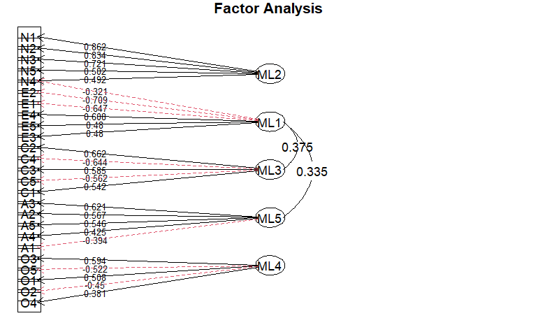
psychパッケージを用いた探索的因子分析のパス図[R]
データ
library(psych)
library(GPArotation)
data(bfi)
d1 <- bfi[1:25]
res01 <- fa(d1, nfactors = 5, fm = "ml", rotate = "promax", scores=TRUE)
fa.diagram (res01, cut=0.3, simple=FALSE, sort=TRUE, digits=3)
オプション
- cut: abs(loading)>cutの負荷が表示される
- simple: 項目ごとの最大荷重のみを表示
- digits: : 係数の桁数
- sort: 因子負荷量をソートしてから図を表示する
- graphviz: 出力にRgraphvizを使うか
過去のpsychパッケージに関するエントリ
https://ides.hatenablog.com/entry/2019/03/19/093726 https://ides.hatenablog.com/entry/2019/04/08/171145 https://ides.hatenablog.com/entry/2019/07/14/160817 https://ides.hatenablog.com/entry/2019/07/31/031654 https://ides.hatenablog.com/entry/2019/08/02/052958
同期交差遅延モデル・測定誤差モデル[Stata]
こちらの続き。
このモデルには2つの新しい特徴がある。まず、相互効果、つまり、ある時間において変数がお互いに影響し合うことができるということである。
波間の係数に等式制約を加えた。例えば、pid2004からapp2004への影響は、(a)pid2002からapp2002への影響と同じになるように制約をかけた。同様に(b)app2004からpid2004への効果は、app2002からpid2002への効果と同じになるように制約をかけた。
3.1 STATA SEMビルダーで、まず矢印を選択し、制約を追加することで、これらの制約を追加することができる。

. sem (pid2000 -> pid2002, ) (pid2000 -> app2002, ) (app2000 -> pid2002, ) ///
(app2000 -> app2002, ) (pid2002@a -> app2002, ) (pid2002 -> pid2004, ) ///
(pid2002 -> app2004, ) (app2002@b -> pid2002, ) (app2002 -> pid2004, ) ///
(app2002 -> app2004, ) (pid2004@a -> app2004, ) (app2004@b -> pid2004, ), standardized cov( app2000*pid2000) nocapslatent

(1069 observations with missing values excluded)

Endogenous variables
  Observed: pid2002 app2002 pid2004 app2004

Exogenous variables
  Observed: pid2000 app2000

Fitting target model:
Iteration 0:   log likelihood =  -7490.988
Iteration 1:   log likelihood = -7390.2964
Iteration 2:   log likelihood = -7385.3207
Iteration 3:   log likelihood = -7385.2859
Iteration 4:   log likelihood = -7385.2859

Structural equation model                                  Number of obs = 738
Estimation method: ml

Log likelihood = -7385.2859

 ( 1)  [pid2002]app2002 - [pid2004]app2004 = 0
 ( 2)  [app2002]pid2002 - [app2004]pid2004 = 0
-------------------------------------------------------------------------------------
                    |                 OIM
       Standardized | Coefficient  std. err.      z    P>|z|     [95% conf. interval]
--------------------+----------------------------------------------------------------
Structural          |
  pid2002           |
            app2002 |   .0597253   .0892213     0.67   0.503    -.1151452    .2345958
            pid2000 |   .7680564   .0420354    18.27   0.000     .6856685    .8504443
            app2000 |   .1188559   .0258264     4.60   0.000     .0682371    .1694747
              _cons |   .0203946   .1418517     0.14   0.886    -.2576296    .2984188
  ------------------+----------------------------------------------------------------
  app2002           |
            pid2002 |   .3984309   .2239883     1.78   0.075     -.040578    .8374399
            pid2000 |   .1090515   .1798212     0.61   0.544    -.2433916    .4614946
            app2000 |   .1042124   .0467443     2.23   0.026     .0125952    .1958296
              _cons |   1.505822   .0853364    17.65   0.000     1.338565    1.673078
  ------------------+----------------------------------------------------------------
  pid2004           |
            pid2002 |    .801487   .0394279    20.33   0.000     .7242096    .8787643
            app2002 |   .0661565   .0509644     1.30   0.194    -.0337319    .1660449
            app2004 |   .0645941   .0962275     0.67   0.502    -.1240084    .2531966
              _cons |   -.084726   .0433142    -1.96   0.050    -.1696203    .0001682
  ------------------+----------------------------------------------------------------
  app2004           |
            pid2002 |   .0686076    .172548     0.40   0.691    -.2695801    .4067954
            app2002 |   .4526101    .034214    13.23   0.000     .3855518    .5196683
            pid2004 |   .3683993   .2055088     1.79   0.073    -.0343905    .7711892
              _cons |   .1497953   .0610446     2.45   0.014     .0301501    .2694405
--------------------+----------------------------------------------------------------
       mean(pid2000)|   1.365443   .0511682    26.69   0.000     1.265155     1.46573
       mean(app2000)|   1.533387   .0542957    28.24   0.000      1.42697    1.639805
--------------------+----------------------------------------------------------------
      var(e.pid2002)|   .2156122   .0211922                       .177832    .2614187
      var(e.app2002)|   .6459226   .0295039                       .590609    .7064167
      var(e.pid2004)|   .2010162   .0199356                       .165506    .2441452
      var(e.app2004)|    .358397    .023088                      .3158856    .4066296
        var(pid2000)|          1          .                             .           .
        var(app2000)|          1          .                             .           .
--------------------+----------------------------------------------------------------
cov(pid2000,app2000)|    .616486   .0228205    27.01   0.000     .5717586    .6612133
-------------------------------------------------------------------------------------
LR test of model vs. saturated: chi2(4) = 133.51                 Prob > chi2 = 0.0000
等値制約をかけたことに表記がある
 ( 1)  [pid2002]app2002 - [pid2004]app2004 = 0
 ( 2)  [app2002]pid2002 - [app2004]pid2004 = 0
. estat gof, sta(all)

----------------------------------------------------------------------------
Fit statistic        |      Value   Description
---------------------+------------------------------------------------------
Likelihood ratio     |
          chi2_ms(4) |    133.511   model vs. saturated
            p > chi2 |      0.000
         chi2_bs(14) |   3458.563   baseline vs. saturated
            p > chi2 |      0.000
---------------------+------------------------------------------------------
Population error     |
               RMSEA |      0.210   Root mean squared error of approximation
 90% CI, lower bound |      0.180
         upper bound |      0.241
              pclose |      0.000   Probability RMSEA <= 0.05
---------------------+------------------------------------------------------
Information criteria |
                 AIC |  14816.572   Akaike's information criterion
                 BIC |  14922.462   Bayesian information criterion
---------------------+------------------------------------------------------
Baseline comparison  |
                 CFI |      0.962   Comparative fit index
                 TLI |      0.868   Tucker–Lewis index
---------------------+------------------------------------------------------
Size of residuals    |
                SRMR |      0.032   Standardized root mean squared residual
                  CD |      0.794   Coefficient of determination
----------------------------------------------------------------------------
4 測定誤差モデル
測定誤差はパネル分析で特に問題となる。SEMのフレームワークでは、この問題を簡単に扱うことができる。たとえば、自己回帰モデルを使って、その測定誤差をモデル化することができます。同定されたモデルを持つために、Wiley-Wiley解をモデル化する(測定誤差が等しいと仮定する)。
このモデルでは、誤差の分散を制約条件として使用する。
これについてはFinkel (1995)に詳しい。 Rで分散共分散行列を得ることができる。 まず、行列を得るために必要な変数を関数 var を使って選択する。 dplyrの関数selectと%>%を使って、一行ですべてを行うようにしよう。
library(dplyr)
new%>%dplyr::select(pid2000,pid2002,pid2004)%>%
  var(na.rm=TRUE)
##          pid2000  pid2002  pid2004
## pid2000 4.681774 4.111523 4.301286
## pid2002 4.111523 4.752644 4.474202
## pid2004 4.301286 4.474202 5.428772
4.75-(4.47*4.11)/4.30
## [1] 0.4775116

round(4.75-(4.47*4.11)/4.30,2)
## [1] 0.48
SEMビルダーを使って、各変数の潜在変数を作成し、その誤差分散を0.48に制約する。

. sem (P2002 -> pid2002, ) (P2002 -> P2004, ) (P2004 -> pid2004, ) (P2000 -> pid2000, ) (P2000 -> P2002, ),
latent(P2002 P2004 P2000 ) cov( e.pid2000@0.48 e.pid2002@0.48 e.pid2004@0.48) nocapslatent
(997 observations with missing values excluded)

Endogenous variables
  Measurement: pid2002 pid2004 pid2000
  Latent:      P2002 P2004

Exogenous variables
  Latent: P2000

Fitting target model:
Iteration 0:   log likelihood = -4293.5454  (not concave)
Iteration 1:   log likelihood = -4212.1818
Iteration 2:   log likelihood = -4160.5424
Iteration 3:   log likelihood = -4150.2215
Iteration 4:   log likelihood =  -4145.957
Iteration 5:   log likelihood = -4145.9269
Iteration 6:   log likelihood = -4145.9269

Structural equation model                                  Number of obs = 810
Estimation method: ml

Log likelihood = -4145.9269

 ( 1)  [pid2002]P2002 = 1
 ( 2)  [pid2004]P2004 = 1
 ( 3)  [pid2000]P2000 = 1
 ( 4)  [/]var(e.pid2002) = .48
 ( 5)  [/]var(e.pid2004) = .48
 ( 6)  [/]var(e.pid2000) = .48
-------------------------------------------------------------------------------
              |                 OIM
              | Coefficient  std. err.      z    P>|z|     [95% conf. interval]
--------------+----------------------------------------------------------------
Structural    |
  P2002       |
        P2000 |    .978417    .020013    48.89   0.000     .9391922    1.017642
  ------------+----------------------------------------------------------------
  P2004       |
        P2002 |   1.046779   .0199761    52.40   0.000     1.007627    1.085932
--------------+----------------------------------------------------------------
Measurement   |
  pid2002     |
        P2002 |          1  (constrained)
        _cons |   3.037037   .0765625    39.67   0.000     2.886977    3.187097
  ------------+----------------------------------------------------------------
  pid2004     |
        P2004 |          1  (constrained)
        _cons |   3.012346   .0818163    36.82   0.000     2.851989    3.172703
  ------------+----------------------------------------------------------------
  pid2000     |
        P2000 |          1  (constrained)
        _cons |   2.925926   .0759792    38.51   0.000      2.77701    3.074842
--------------+----------------------------------------------------------------
var(e.pid2002)|        .48  (constrained)
var(e.pid2004)|        .48  (constrained)
var(e.pid2000)|        .48  (constrained)
  var(e.P2002)|   .2512405   .0500669                      .1700057    .3712923
  var(e.P2004)|   .2653503   .0539494                      .1781389     .395258
    var(P2000)|   4.195995    .232352                      3.764436    4.677028
-------------------------------------------------------------------------------
LR test of model vs. saturated: chi2(1) = 0.01             Prob > chi2 = 0.9173
磯村毅、ESS(電子スクリーン症候群)、スマホ依存防止学会、疑似科学
ASDは先天的な脳の一部の障害だが、症状の程度は、育った環境の影響を受けるといわれている。つまり、先天的に自閉症スペクトラムを持っている子供は、スクリーンタイムが長いと、その症状が悪化する傾向にあるのだ。さらに、その傾向は、生まれつき自閉症を抱えていない子供にも表れることがある。スマホ依存防止学会代表の磯村毅さんが言う。
「『ESS(電子スクリーン症候群)』といって、スマホやタブレットなどの画面からの刺激で子供の脳が変調し、発達障害やうつ、双極性障害などに似た症状が出ることがあります。
プロのゲーマーになるほどスクリーンの刺激に強い子がいる一方、友達から借りたゲーム機で少し遊ぶだけで、発達障害と間違えられるほど落ち着きがなくなる子や、学校でデジタル黒板が導入されたとたんに頭痛とチックが起こって成績が落ちる子もいる。スクリーンの刺激に強いか弱いかは、一人ひとり異なるのです」(磯村さん・以下同)
スマホ依存防止学会
ESSリセット研究会
磯村毅
代表 磯村毅
医師
もともとは呼吸器科医です。子どもの禁煙支援が専門で、依存症の脳科学に興味を持ち、現在はスマホ依存に取り組んでいます。
NHKのためしてガッテンに出たことが自慢。
「リセット禁煙」「二重洗脳」「親子で読むケータイ依存脱出法」などの著書もあります。日本動機づけ面接学会代表理事
( ´_ゝ`)フーン
事務局所在地
〒182-0001 東京調布市緑ヶ丘2−5−2
副代表・事務局の清水俊貴さんの歯科医院に事務局があるようだ。
スマホ依存防止アドバイザー講座
スマホ依存防止 アドバイザー
地域別 PISA認定アドバイザー数 ( 人 )
北海道/東北 14 (北海道 3, 青森 4, 岩手 0, 宮城 3, 秋田 1, 山形 2, 福島 1 )
関東 31 (茨城 1, 栃木 0. 群馬 0, 埼玉 1, 千葉 5, 東京 16, 神奈川 7 )
中部 67 (新潟 3, 富山 1, 石川 2, 福井 4, 山梨 6, 長野 2, 岐阜 2, 静岡 3, 愛知 44 )
近畿 11 (三重 3. 滋賀 1, 京都 2, 大阪 1, 兵庫 1. 奈良 2, 和歌山 1 )
中国 12 (鳥取 3, 島根 0, 岡山 1, 広島 4, 山口 4 )
四国 2 (徳島 0, 香川 1, 愛媛 0, 高知 1 )
九州/沖縄 56 (福岡 22, 佐賀 0, 長崎 0, 熊本 17, 大分 1, 宮崎 7, 鹿児島 7, 沖縄 2)
(高校生3名 大学生1名を含む)
資格商売を始めたいようだ。
電子スクリーン症候群 Electronic Screen Syndromeの科学的エビデンス
もちろんゼロである。疑似科学である。
ロート製薬も何かを始めている
UMINに登録があった。
主要アウトカム評価項目が電子スクリーンの有無による脳波特徴量検出になっている。 どうやって金儲けにつなげるのか、興味があるところだ。
自己回帰モデルと交差遅延パネルモデル[Stata]
こちらから。
データはこちらに上がっているようだ。
1.自己回帰モデル
3波を自己回帰させる。
use "nes3wave.dta", clear
GUI


最尤法で実行。

CUI
sem (pid2000 -> pid2002, ) (pid2002 -> pid2004, ), nocapslatent
オプション
- latent(names)...潜在的な変数名を明示的に指定する。
latent(names) は names が潜在変数の名前の完全な集合であることを指定する。 sem と gsem は通常、潜在変数の最初の文字を大文字にし、観測変数の最初の文字を小文字にすると仮定する; [SEM] sem とsemのパス表記を参照されたい。 semのパス表記を参照。 latent(names) を指定すると、sem と gsem は、リストされた変数を潜在変数として扱い、それ以外の変数は、大文字小文字にかかわらず、観測された変数として扱う。
- nocapslatent...大文字を潜在的なものとして扱わない。
nocapslatent は、最初の文字が大文字であることは、潜在変数を指定しないことを指定する。 このオプションは、データセット内のいくつかの観測変数が最初の文字を大文字にしている場合に、観測変数のみでモデルをフィットするときに使用することができる。
. sem (pid2000 -> pid2002, ) (pid2002 -> pid2004, ), nocapslatent
(997 observations with missing values excluded)

Endogenous variables
  Observed: pid2002 pid2004

Exogenous variables
  Observed: pid2000

Fitting target model:
Iteration 0:   log likelihood = -4204.8919
Iteration 1:   log likelihood = -4204.8919

Structural equation model                                  Number of obs = 810
Estimation method: ml

Log likelihood = -4204.8919

-------------------------------------------------------------------------------
              |                 OIM
              | Coefficient  std. err.      z    P>|z|     [95% conf. interval]
--------------+----------------------------------------------------------------
Structural    |
  pid2002     |
      pid2000 |   .8781976   .0173528    50.61   0.000     .8441868    .9122084
        _cons |   .4674959   .0631342     7.40   0.000     .3437552    .5912366
  ------------+----------------------------------------------------------------
  pid2004     |
      pid2002 |   .9414133   .0177779    52.95   0.000     .9065692    .9762574
        _cons |   .1532385   .0664485     2.31   0.021     .0230019    .2834752
--------------+----------------------------------------------------------------
var(e.pid2002)|   1.140504   .0566721                      1.034667    1.257168
var(e.pid2004)|   1.215196   .0603836                      1.102427    1.339501
-------------------------------------------------------------------------------
LR test of model vs. saturated: chi2(1) = 117.94           Prob > chi2 = 0.0000
SEMモデルには適合度測定が重要である。STATAでモデルを推定した後、estat gof, sta(all)を実行すると、それを得ることができる。
. estat gof, sta(all)

----------------------------------------------------------------------------
Fit statistic        |      Value   Description
---------------------+------------------------------------------------------
Likelihood ratio     |
          chi2_ms(1) |    117.941   model vs. saturated
            p > chi2 |      0.000
          chi2_bs(3) |   2484.410   baseline vs. saturated
            p > chi2 |      0.000
---------------------+------------------------------------------------------
Population error     |
               RMSEA |      0.380   Root mean squared error of approximation
 90% CI, lower bound |      0.324
         upper bound |      0.440
              pclose |      0.000   Probability RMSEA <= 0.05
---------------------+------------------------------------------------------
Information criteria |
                 AIC |   8421.784   Akaike's information criterion
                 BIC |   8449.966   Bayesian information criterion
---------------------+------------------------------------------------------
Baseline comparison  |
                 CFI |      0.953   Comparative fit index
                 TLI |      0.859   Tucker–Lewis index
---------------------+------------------------------------------------------
Size of residuals    |
                SRMR |      0.035   Standardized root mean squared residual
                  CD |      0.760   Coefficient of determination
----------------------------------------------------------------------------
交差遅延モデル Cross-lagged models
GUI

CUI
. sem (pid2000 -> pid2002, ) (pid2000 -> app2002, ) //
 (app2000 -> pid2002, ) (app2000 -> app2002, ),
 standardized cov( pid2000*app2000) nocapslatent//

(748 observations with missing values excluded)

Endogenous variables
  Observed: pid2002 app2002

Exogenous variables
  Observed: pid2000 app2000

Fitting target model:
Iteration 0:   log likelihood = -7560.2496
Iteration 1:   log likelihood = -7560.2496  (backed up)

Structural equation model                                Number of obs = 1,059
Estimation method: ml

Log likelihood = -7560.2496

-------------------------------------------------------------------------------------
                    |                 OIM
       Standardized | Coefficient  std. err.      z    P>|z|     [95% conf. interval]
--------------------+----------------------------------------------------------------
Structural          |
  pid2002           |
            pid2000 |   .7729582   .0158919    48.64   0.000     .7418106    .8041057
            app2000 |   .1241617   .0200544     6.19   0.000     .0848557    .1634676
              _cons |   .1624004   .0322593     5.03   0.000     .0991733    .2256274
  ------------------+----------------------------------------------------------------
  app2002           |
            pid2000 |   .4239438   .0308988    13.72   0.000     .3633831    .4845044
            app2000 |   .1370873   .0326491     4.20   0.000     .0730961    .2010784
              _cons |   1.558611    .072866    21.39   0.000     1.415797    1.701426
--------------------+----------------------------------------------------------------
       mean(pid2000)|   1.339711   .0423285    31.65   0.000     1.256749    1.422674
       mean(app2000)|   1.521585   .0451376    33.71   0.000     1.433117    1.610053
--------------------+----------------------------------------------------------------
      var(e.pid2002)|   .2722378   .0142733                       .245652    .3017009
      var(e.app2002)|   .7319102   .0232906                      .6876559    .7790124
        var(pid2000)|          1          .                             .           .
        var(app2000)|          1          .                             .           .
--------------------+----------------------------------------------------------------
cov(pid2000,app2000)|   .5985186   .0197213    30.35   0.000     .5598656    .6371716
-------------------------------------------------------------------------------------
LR test of model vs. saturated: chi2(1) = 90.40                  Prob > chi2 = 0.0000
適合度。
. estat gof, sta(all)

----------------------------------------------------------------------------
Fit statistic        |      Value   Description
---------------------+------------------------------------------------------
Likelihood ratio     |
          chi2_ms(1) |     90.399   model vs. saturated
            p > chi2 |      0.000
          chi2_bs(5) |   1798.754   baseline vs. saturated
            p > chi2 |      0.000
---------------------+------------------------------------------------------
Population error     |
               RMSEA |      0.291   Root mean squared error of approximation
 90% CI, lower bound |      0.242
         upper bound |      0.343
              pclose |      0.000   Probability RMSEA <= 0.05
---------------------+------------------------------------------------------
Information criteria |
                 AIC |  15146.499   Akaike's information criterion
                 BIC |  15211.045   Bayesian information criterion
---------------------+------------------------------------------------------
Baseline comparison  |
                 CFI |      0.950   Comparative fit index
                 TLI |      0.751   Tucker–Lewis index
---------------------+------------------------------------------------------
Size of residuals    |
                SRMR |      0.040   Standardized root mean squared residual
                  CD |      0.753   Coefficient of determination
----------------------------------------------------------------------------
パネルデータ分析における固定効果およびランダム効果[Stata]
Sayed HossainさんのYouTube動画から。
データはこちらからダウンロードできる。 https://bityl.co/E3kh
以下の手法でパネルデータを作成する。
- プールドOLS回帰モデル
- 固定効果モデルまたはLSDVモデル
- ランダム効果モデル
データ

ここでは、111, 222, 333, 444, 555, 666の6つのコンピュータ会社を取り上げ、コンピュータの販売台数、コンピュータの価格、コンピュータの修理の3つの変数を持っている。ここでは、売上高と他の2つの説明変数(価格、修理費)の関係を調べる。 データは、2000年から2010年まで。したがって、我々の観測値は66となる。
3つのモデル
pooled regression プールド回帰 ここでは、66の観測値をすべてプールし、データの横断的、時系列的な性質を無視して回帰モデルを実行する。 このモデルの大きな問題点は、様々なコンピュータ会社を区別していないことです。言い換えれば、プールによって6つの会社を組み合わせることで、6つのコンピュータ会社の間に存在するかもしれない異質性や個性を否定していることになる。
固定効果モデルまたは LSDV モデル 固定効果モデルまたはLSDVモデルLeast Square Dummy Variable (Regress with group dummies) は、独自の切片値を持たせることによって、6つのコンピュータ会社間の異質性または個別性を許容するものである。 固定効果という言葉は、切片はコンピュータ会社間で異なるかもしれないが、切片は時間的に変化しない、つまり時間不変であるという事実に起因するものである。
ランダム効果モデル ここでは、6社は切片の平均値が共通である。 ここで、どのモデル(固定効果またはランダム効果)を受け入れるのが適切かを確認するために、Hausman 検定を適用することにする。
ハウスマン検定 Hausman Test
帰無仮説: ランダム効果モデルが適切 対立仮説: 固定効果モデルが適切である 統計的に有意なP値が得られたら固定効果モデル、そうでなければランダム効果モデルを使う。
診断チェック
最後に、残差に系列相関があるかどうかを確認することにする。ここでは、Pasaran CD (cross-sectional dependence)検定を用いて、残差に主体間の相関があるかどうかを検定することにする。 Null:系列相関がない。 Alt: 系列相関がある。
データのインポート
. import excel "Panel_Data._Model_One._STATA.xlsx", sheet("Sheet1") firstrow
pooled regression
売り上げ Sales を従属変数、 価格 Price と修理 Repairs を独立変数にする。
. regress Sales Price Repairs

      Source |       SS           df       MS      Number of obs   =        66
-------------+----------------------------------   F(2, 63)        =      4.10
       Model |  3.6436e+11         2  1.8218e+11   Prob > F        =    0.0212
    Residual |  2.7986e+12        63  4.4422e+10   R-squared       =    0.1152
-------------+----------------------------------   Adj R-squared   =    0.0871
       Total |  3.1630e+12        65  4.8661e+10   Root MSE        =    2.1e+05

------------------------------------------------------------------------------
       Sales | Coefficient  Std. err.      t    P>|t|     [95% conf. interval]
-------------+----------------------------------------------------------------
       Price |   1050.312    391.932     2.68   0.009     267.0987    1833.526
     Repairs |   8.831223   7.370528     1.20   0.235    -5.897602    23.56005
       _cons |  -212624.6   163259.5    -1.30   0.198    -538872.7    113623.5
------------------------------------------------------------------------------
6社に違いはないという仮定に基づくモデル。 価格 Price のみが有意な変数という結果である。
パネル変数と時間変数を設定する。
パネルは会社、時間は年で設定する。
. xtset CompanyCode YEAR

Panel variable: CompanyCode (strongly balanced)
 Time variable: YEAR, 2000 to 2010
         Delta: 1 unit
固定効果モデル
xtregコマンドにFixed Mdelの頭文字feをつける。
. xtreg Sales Price Repairs, fe

Fixed-effects (within) regression               Number of obs     =         66
Group variable: CompanyCode                     Number of groups  =          6

R-squared:                                      Obs per group:
     Within  = 0.2075                                         min =         11
     Between = 0.0863                                         avg =       11.0
     Overall = 0.0847                                         max =         11

                                                F(2,58)           =       7.59
corr(u_i, Xb) = 0.1577                          Prob > F          =     0.0012

------------------------------------------------------------------------------
       Sales | Coefficient  Std. err.      t    P>|t|     [95% conf. interval]
-------------+----------------------------------------------------------------
       Price |   285.1704   73.27324     3.89   0.000      138.498    431.8427
     Repairs |  -.9394111    5.34654    -0.18   0.861    -11.64167    9.762851
       _cons |   95663.84   34678.16     2.76   0.008     26247.97    165079.7
-------------+----------------------------------------------------------------
     sigma_u |  231289.36
     sigma_e |  21203.939
         rho |  .99166536   (fraction of variance due to u_i)
------------------------------------------------------------------------------
F test that all u_i=0: F(5, 58) = 1233.32                    Prob > F = 0.0000
Prob > F = 0.0012と5%未満であることからモデルのフィットは悪くないことがわかる。
モデルの保存
のちのち比較するためモデルを保存しておく必要がある。Fixedという名前で保存することにする。
estimates store Fixed
ランダム効果モデル
Randam Effect GLSでの推定値。
. xtreg Sales Price Repairs, re

Random-effects GLS regression                   Number of obs     =         66
Group variable: CompanyCode                     Number of groups  =          6

R-squared:                                      Obs per group:
     Within  = 0.2075                                         min =         11
     Between = 0.0860                                         avg =       11.0
     Overall = 0.0844                                         max =         11

                                                Wald chi2(2)      =      15.83
corr(u_i, X) = 0 (assumed)                      Prob > chi2       =     0.0004

------------------------------------------------------------------------------
       Sales | Coefficient  Std. err.      z    P>|z|     [95% conf. interval]
-------------+----------------------------------------------------------------
       Price |   286.5764   72.07584     3.98   0.000     145.3103    427.8424
     Repairs |  -.9714552    5.13579    -0.19   0.850    -11.03742    9.094508
       _cons |   95345.83   119938.4     0.79   0.427    -139729.1    330420.8
-------------+----------------------------------------------------------------
     sigma_u |  285744.06
     sigma_e |  21203.939
         rho |  .99452362   (fraction of variance due to u_i)
------------------------------------------------------------------------------
Prob > F = 0.0004と5%未満であることからモデルのフィットは悪くないことがわかる。
モデルの保存
estimates store Random
ハウスマン検定
固定効果モデルで推定したFixedをハウスマン検定にかける。
. hausman Fixed

                 ---- Coefficients ----
             |      (b)          (B)            (b-B)     sqrt(diag(V_b-V_B))
             |     Fixed        Random       Difference       Std. err.
-------------+----------------------------------------------------------------
       Price |    285.1704     286.5764       -1.405973         13.1925
     Repairs |   -.9394111    -.9714552        .0320441         1.48632
------------------------------------------------------------------------------
                          b = Consistent under H0 and Ha; obtained from xtreg.
           B = Inconsistent under Ha, efficient under H0; obtained from xtreg.

Test of H0: Difference in coefficients not systematic

    chi2(2) = (b-B)'[(V_b-V_B)^(-1)](b-B)
            =   0.01
Prob > chi2 = 0.9942
カイ二乗検定の結果は Prob > chi2 = 0.9942 であり、5%有意ではない。 帰無仮説は棄却しないため、ランダム効果モデルが適切ということなる。
残差の系列相関のチェック
パッケージst0113のインストールが必要のようだ。
net install st0113.pkg
Pasaran CD (cross-sectional dependence)検定を行う。
. xtcsd, pesaran abs

Pesaran's test of cross sectional independence =     0.956, Pr = 0.3391

Average absolute value of the off-diagonal elements =     0.553
有意確率はPr = 0.3391であり、5%有意ではない。帰無仮説は「系列相関がない」であるため、系列相関を考えなくてもよいことがわかった。
皮膚むしり症 Excoriation Disorderの評価
こちらの論文から先行研究の整理。
皮膚むしり症 Excoriation Disorder は、1875年にErasmus Wilsonによって、神経症患者の制御が不可能ではないにしても困難な過剰な皮膚摘出行動を指して、「neurotic excoriation」(Wilson,1875)という名称で記述された(Torales et al.,2020)。この疾患は、強迫性スキンピッキング、病的スキンピッキング、心因性排泄、またはdermatillomaniaなどの他の呼称を受けている(Lochner et al.、2017)。EDは、皮膚を繰り返し摘み、皮膚病変や重大な苦痛または機能障害につながるものとして説明される。この障害に罹患した患者は、典型的な病変が現れるまで、これらの行為を強迫的に行わなければならないと感じる(Jafferany & Patel, 2019; Torales et al, 2019)。この障害は、「精神障害の診断と統計マニュアル」(DSM-5)第5版の強迫性障害およびその他の関連障害の章に分類されている(米国精神医学会、2013年)。
皮膚むしり症 Excoriation Disorder:EDの推定有病率は1%~5%と報告されており(Russell et al.、2020)、成人期(30~45歳)に発症のピークを迎える(Rivera & Arenas、2016)。
- Torales, J., Ruiz Díaz, N., Barrios, I., Navarro, R., García, O., O’Higgins, M., CastaldelliMaia, J. M., Ventriglio, A., & Jafferany, M. (2020). Psychodermatology of skin picking (excoriation disorder): A comprehensive review. Dermatologic Therapy, 33 (4), Article e13661. https://doi.org/10.1111/dth.13661
https://onlinelibrary.wiley.com/doi/10.1111/dth.13661
- Çalıkus ̧u, C., Yücel, B., Polat, A., & Baykal, C. (2003). The relation of psychogenic excoriation with psychiatric disorders: A comparative study. Comprehensive Psychiatry, 44(3), 256–261. https://doi.org/10.1016/S0010-440X(03)00041-5
女性がより影響を受けやすいとされている(Grant et al.、2011)。
- Grant, J. E., Odlaug, B. L., & Chamberlain, S. R. (2011). A cognitive comparison of pathological skin picking and trichotillomania. Journal of Psychiatric Research, 45 (12), 1634–1638. https://doi.org/10.1016/j.jpsychires.2011.07.012
臨床的には、EDは顕著な異質性と現象的複雑性を示し、重大な感情的・身体的影響を伴う(Odlaug & Grant, 2012)。しかしながら、ED患者にはいくつかの要素が習慣的に観察される(表1)(Stein et al., 2010)。
| 表1 ED患者に必ず見られる3つの要素 |
|---|
| 組織損傷、出血、または痛みを引き起こす、再発性のある皮膚の摘出。 |
| 皮膚をほじることによって生じる重大な不快感または障害、および。 |
| その行動が他の医学的、精神医学的疾患や物質使用によるものではないこと(例:皮膚科疾患、身体醜形障害、アンフェタミン使用、など各々)。 |
- Stein, D. J., Grant, J. E., Franklin, M. E., Keuthen, N., Lochner, C., Singer, H. S., & Woods, D. W. (2010). Trichotillomania (hair pulling disorder), skin picking disorder, and stereotypic movement disorder: Toward DSM-V. Depression and Anxiety, 27(6), 611–626. https://doi.org/10.1002/da.20700
https://onlinelibrary.wiley.com/doi/10.1002/da.20700
EDの評価は、臨床医が実施する評価尺度や自己申告による評価尺度に基づいて行われる(Barrios et al.、2020)。
- Barrios, I., Jafferany, M., Ruiz Díaz, N., Castaldelli-Maia, J. M., Ventriglio, A., & Torales, J. (2020). Psychometric properties of the Spanish version of the skin picking scale-revised (SPS-R). Journal of Obsessive-Compulsive and Related Disorders, 27, 100586. https://doi.org/10.1016/j.jocrd.2020.100586
臨床家評価尺度のうち、神経性皮膚むしり症用に修正したYale-Brown Obsessive-Compulsive ScaleとSkin Picking Treatment Scaleがある(Keuthen et al.2012)。
- Keuthen, N., Siev, J., & Reese, H. (2012). Assessment of trichotillomania, pathological skin picking, and stereotypic movement disorder. In E. J. Grant, D. Stein, D. Woods, & N. Keuthen (Eds.), Trichotillomania, skin picking and other body-focused repetitive behaviors (pp. 129–150). American Psychiatric Publishing.

Skin Picking Scale(SPS)とSkin Picking Impact Scale(SPIS)は、EDのための自己記入式尺度であり、それぞれ障害の臨床的重症度と心理社会的影響を測定する(Barrios et al.、2020; Snorrason et al.、2012)。
- Barrios et al.、2020, https://doi.org/10.1016/j.jocrd.2020.100586
- Snorrason, I., ́ Olafsson, R. P., Flessner, C. A., Keuthen, N. J., Franklin, M. E., & Woods, D. W. (2012). The skin picking scale-revised: Factor structure and psychometric properties. Journal of Obsessive-Compulsive and Related Disorders, 1(2), 133–137. https://doi.org/10.1016/j.jocrd.2012.03.001
自己記入式尺度は、高い心理測定的妥当性が報告されている(Keuthen et al.、2012)。 ED患者を正しく評価することで、オーダーメイドの治療法につながる可能性があることは注目される。2013年,DSM-5の強迫スペクトラム障害サブワーキンググループは,過去1週間に生じたED症状を問う次元評価として,Excoriation(skin-picking disorder)Dimensional Scale(SPD-D)を開発した(LeBeau et al.,2013)。
- LeBeau, R. T., Mischel, E. R., Simpson, H. B., Mataix-Cols, D., Phillips, K. A., Stein, D. J., & Craske, M. G. (2013). Preliminary assessment of obsessive–compulsive spectrum disorder scales for DSM-5. Journal of Obsessive-Compulsive and Related Disorders, 2(2), 114–118. https://doi.org/10.1016/j.jocrd.2013.01.005