epitoolsパッケージを用いた直接法による年齢標準化(調整)率および「正確な」信頼区間の算出。
こちらの例から。
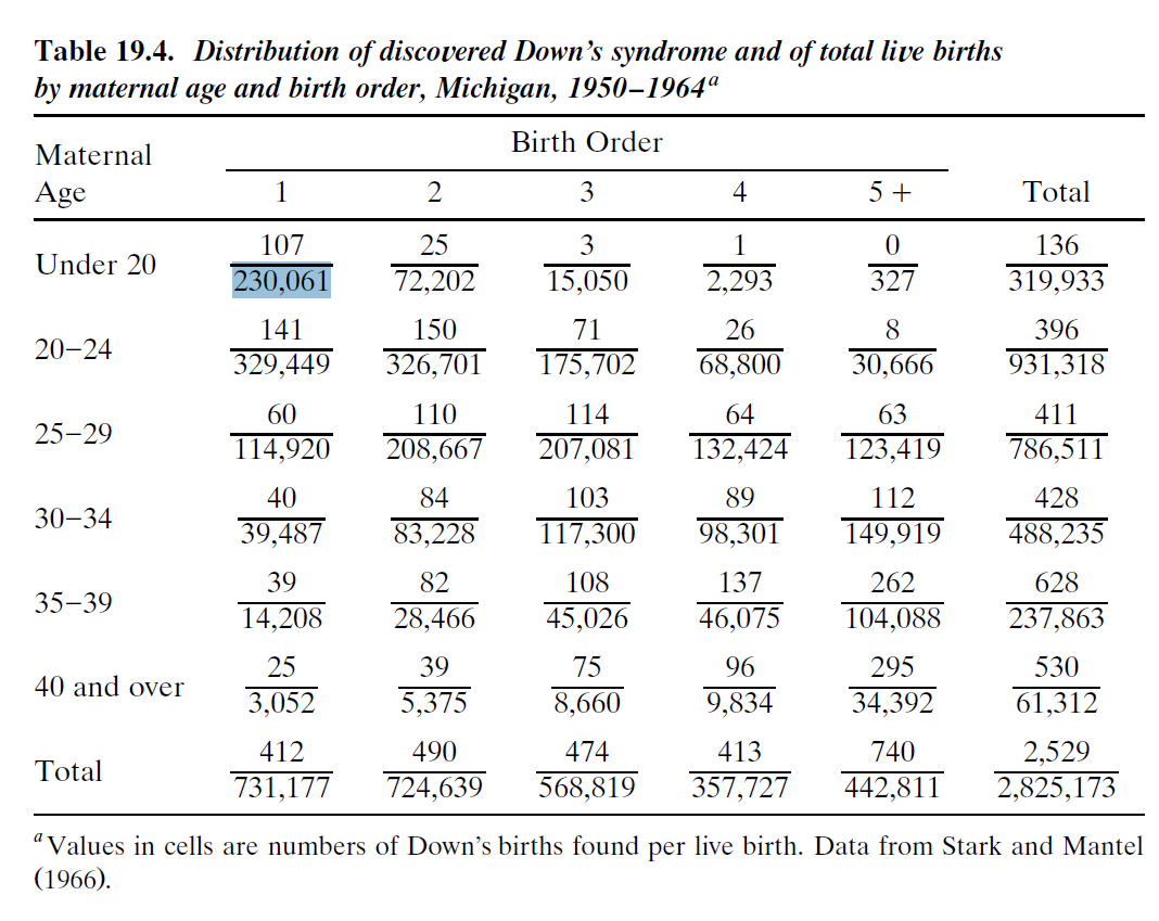
データはこの本からとられている。
 (English Edition)")
3版、640ページの表。
詳細
異なるグループ(地域、民族など)の率を有効に比較するためには、しばしば年齢分布の違いを調整して、年齢による交絡の影響を取り除く必要がある。イベント数や率が非常に少ない場合(地域研究ではよくあること)、信頼区間を計算する通常の近似法では、信頼下限が負の値になることがある。この一般的な落とし穴を避けるために、正確な信頼区間を近似することができる。この関数はこの方法を実装している(Fay 1997)。オリジナルの関数はTJ Aragonによって書かれ、Anderson, 1998に基づいている。この関数は、MP Fayにより、Fay 1998に基づいて書き直され、改良された。
library(epitools)
## Data from Fleiss, 1981, p. 249/ 3rd version 2003, p. 640
population <-
  c(230061, 329449, 114920, 39487, 14208, 3052,
    72202, 326701, 208667, 83228, 28466, 5375, 15050, 175702,
    207081, 117300, 45026, 8660, 2293, 68800, 132424, 98301,
    46075, 9834, 327, 30666, 123419, 149919, 104088, 34392,
    319933, 931318, 786511, 488235, 237863, 61313)
population <- matrix(population, 6, 6,
dimnames = list(c("Under 20", "20-24", "25-29", "30-34", "35-39",
"40 and over"), c("1", "2", "3", "4", "5+", "Total")))
population
populationデータ。
                 1      2      3      4     5+  Total
Under 20    230061  72202  15050   2293    327 319933
20-24       329449 326701 175702  68800  30666 931318
25-29       114920 208667 207081 132424 123419 786511
30-34        39487  83228 117300  98301 149919 488235
35-39        14208  28466  45026  46075 104088 237863
40 and over   3052   5375   8660   9834  34392  61313
count <-
  c(107, 141, 60, 40, 39, 25, 25, 150, 110, 84, 82, 39,
    3, 71, 114, 103, 108, 75, 1, 26, 64, 89, 137, 96, 0, 8, 63, 112,
    262, 295, 136, 396, 411, 428, 628, 530)
count <- matrix(count, 6, 6,
                dimnames = list(c("Under 20", "20-24", "25-29", "30-34", "35-39",
                "40 and over"), c("1", "2", "3", "4", "5+", "Total")))
count
countデータ。
              1   2   3   4  5+ Total
Under 20    107  25   3   1   0   136
20-24       141 150  71  26   8   396
25-29        60 110 114  64  63   411
30-34        40  84 103  89 112   428
35-39        39  82 108 137 262   628
40 and over  25  39  75  96 295   530
平均人口を基準とする
standard<-apply(population[,-6], 1, mean)
standard
年齢階級別の平均値
   Under 20       20-24       25-29       30-34       35-39 40 and over
    63986.6    186263.6    157302.2     97647.0     47572.6     12262.6
Fay and Feuer, 1997の表1の再現
ageadjust.direct()を用いる。
stdpopのデフォルトは0.95。
birth.order1<-ageadjust.direct(count[,1],population[,1],stdpop=standard)
round(10^5*birth.order1,1)

birth.order2<-ageadjust.direct(count[,2],population[,2],stdpop=standard)
round(10^5*birth.order2,1)

birth.order3<-ageadjust.direct(count[,3],population[,3],stdpop=standard)
round(10^5*birth.order3,1)

birth.order4<-ageadjust.direct(count[,4],population[,4],stdpop=standard)
round(10^5*birth.order4,1)

birth.order5p<-ageadjust.direct(count[,5],population[,5],stdpop=standard)
round(10^5*birth.order5p,1)
crude.rate   adj.rate        lci        uci
      56.3       92.3       80.4      105.8
crude.rate   adj.rate        lci        uci
      67.6       91.2       82.4      100.9
crude.rate   adj.rate        lci        uci
      83.3       85.1       77.2       94.2
crude.rate   adj.rate        lci        uci
     115.5       92.7       80.0      114.7
crude.rate   adj.rate        lci        uci
     167.1       75.5       67.7      188.3
crude.rate
粗(未調整)レート
adj.rate
年齢調整後のレート
lci
下限信頼区間限界
UCI
上側信頼区間限界
参考文献
Fay MP, Feuer EJ. Confidence intervals for directly standardized rates: a method based on the gamma distribution. Stat Med. 1997 Apr 15;16(7):791-801. PMID: 9131766 Steve Selvin. Statistical Analysis of Epidemiologic Data (Monographs in Epidemiology and Biostatistics, V. 35), Oxford University Press; 3rd edition (May 1, 2004) Anderson RN, Rosenberg HM. Age Standardization of Death Rates: Implementation of the Year 200 Standard. National Vital Statistics Reports; Vol 47 No. 3. Hyattsville, Maryland: National Center for Health Statistics. 1998, pp. 13-19. Available at http://www.cdc.gov/nchs/data/nvsr/nvsr47/nvs47_03.pdf.