Stataでの分析方法はこちら。
Mplusでの分析方法はこちら。
データ読み込み
library(rio)
nes3wave <-import("nes3wave.dta")
今回のパス図を先に表示しておこう。
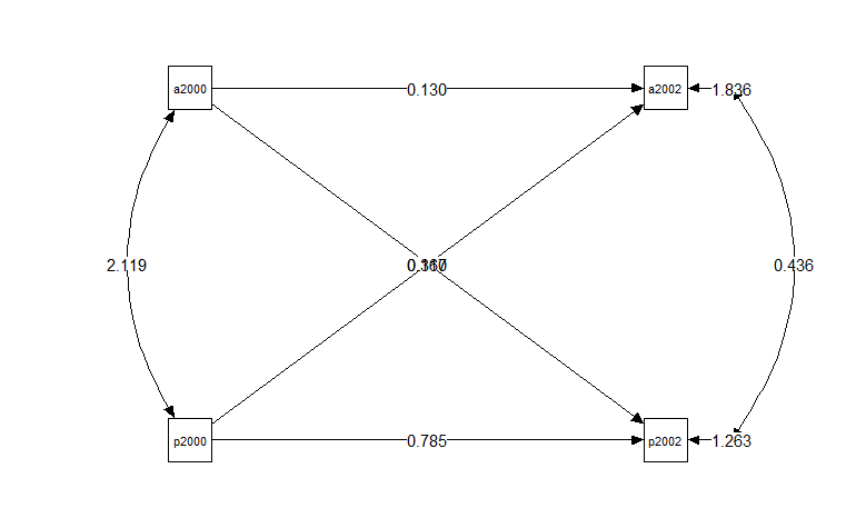
コードは末尾。semPlotパッケージを用いて描画している。
モデル
回帰は~、共変量は~~で書くのがlavaan。
library(lavaan)
CLP_model<-
  '
## Regressions
pid2002 ~ pid2000 + app2000
app2002 ~ app2000 + pid2000

## Covariances
app2000~~pid2000
app2002~~pid2002
'
実行・結果表示
推定法はデフォルトの最尤法を用いている。
fit_CLPM<- sem(CLP_model, data=nes3wave)
summary(fit_CLPM, standardized=TRUE)
結果
Regressions:
                   Estimate  Std.Err  z-value  P(>|z|)   Std.lv  Std.all
  pid2002 ~
    pid2000           0.785    0.020   38.621    0.000    0.785    0.773
    app2000           0.160    0.026    6.204    0.000    0.160    0.124
  app2002 ~
    app2000           0.130    0.031    4.177    0.000    0.130    0.137
    pid2000           0.317    0.025   12.919    0.000    0.317    0.424

Covariances:
                   Estimate  Std.Err  z-value  P(>|z|)   Std.lv  Std.all
  pid2000 ~~
    app2000           2.119    0.127   16.712    0.000    2.119    0.599
 .pid2002 ~~
   .app2002           0.436    0.049    8.950    0.000    0.436    0.286

Variances:
                   Estimate  Std.Err  z-value  P(>|z|)   Std.lv  Std.all
   .pid2002           1.263    0.055   23.011    0.000    1.263    0.272
   .app2002           1.836    0.080   23.011    0.000    1.836    0.732
    pid2000           4.501    0.196   23.011    0.000    4.501    1.000
    app2000           2.785    0.121   23.011    0.000    2.785    1.000
パス図
library(semPlot)
semPaths(fit_CLPM, layout = "tree", shapeLat="ellipse", whatLabels  = "est",
         nDigits=3, shapeMan="square", sizeMan =6, sizeMan2= 10,
         style = "lisrel",rotation = 2,residScale=12, curve=2.5,
         edge.color="black", edge.label.cex=1)
