ベイジアンt検定[R]

www.sumsar.net

bayes.t.test 関数

t.test関数は、4つのバージョンのt検定を実行するために使われる。ここでは、1標本と対の標本の選択肢だけを紹介する。bayes.t.testはt検定のベイジアン的な代替法を実行し、t.test関数と互換性のある関数用法を有している。つまり、t.test(x, conf.int=0.8,mu=1)のようにt-testを実行するだけなら、bayes.を前置するだけですぐに動作するはずである。

bayes.t.testの例として、2002年のNature誌の論文The Value of Bees to the Coffee Harvest (doi:10.1038/417708a, pdf)から引用する。この論文で David W. Roubik は、「熱帯農業の柱である自家受粉のアフリカの低木 Coffea arabicaは昆虫による受粉からは何も得られないと考えられていた」にもかかわらず、ハチはコーヒー収穫にとって重要であると論じている。その論拠となるのが、アフリカミツバチが定着する前の1961年から1980年と、アフリカミツバチがほぼ帰化した1981年から2001年の新世界各国のコーヒー平均収穫量（kg / 10,000m）データである。このデータはミツバチ導入後の収量の増加を示しており、一対の t 検定で分析すると p = 0.04という結果になる。これは、ミツバチがずっと忙しく飛び回っていた旧世界の国々での収穫量の増加と比較すると、一対のt検定ではp =0.232となり、「変化なし」と解釈される。データセットは以下の表とcsvファイル（論文での分析に合わせるため、csvファイルにはカリブ海の島々は含まれていない）にある。

https://www.sumsar.net/files/posts/2014-02-04-bayesian-first-aid-one-sample-t-test/roubik_2002_coffe_yield.csv

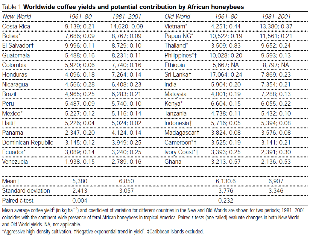
このデータセットの分析にt検定を用いることが適切でない理由はいくつかある。t-testでは、各国の地理的な位置は考慮されていないし、どのような「集団」から抽出されたサンプルなのかも明らかではない。また、「相関関係は因果関係を意味しない」という古い決まり文句を唱えたくもなる。確かに、1961年と2001年の間にボリビアで変わったことは、ミツバチの導入以外にたくさんあるはずだ。このような反論を承知で、それでも私は、対応のあるbayes.t.testを紹介するために、この論文を使うつもりである。

まず、論文のオリジナル分析を実行しよう。

d <- read.csv("https://www.sumsar.net/files/posts/2014-02-04-bayesian-first-aid-one-sample-t-test/roubik_2002_coffe_yield.csv")
new_yield_80 <- d$yield_61_to_80[d$world == "new"]
new_yield_01 <- d$yield_81_to_01[d$world == "new"]
t.test(new_yield_01, new_yield_80, paired = TRUE, alternative = "greater")

 Paired t-test

data:  new_yield_01 and new_yield_80
t = 3.1156, df = 12, p-value = 0.004464
alternative hypothesis: true difference in means is greater than 0
95 percent confidence interval:
 628.9914      Inf
sample estimates:
mean of the differences 
               1469.769 

この論文では、片側t検定を使っているので、信頼区間が広くなっている。

では、ベイズ的応急処置の代替案だ。

パッケージのインストール

BayesianFirstAid()はJAGSを用いる。rjags()のインストールが必要だ。

install.packages("rjags")

rjags()のインストールがうまくいかない場合にはこちらを参照のこと。
https://gist.github.com/casallas/8411082

Githubからのインストールに必要なdevtools()をインストールしていない場合には、まずインストールが必要である。

install.packages("devtools")

次にGithubからBayesianFirstAid()をインストールする

devtools::install_github("rasmusab/bayesian_first_aid")

BayesianFirstAid()でのベイジアンT検定

library(BayesianFirstAid)
bayes.t.test(new_yield_01, new_yield_80, paired = TRUE, alternative = "less")

 Bayesian estimation supersedes the t test (BEST) - paired samples

data: new_yield_01 and new_yield_80, n = 13

  Estimates [95% credible interval]
mean paired difference: 1402 [376, 2441]
sd of the paired differences: 1688 [895, 2698]

The mean difference is more than 0 by a probability of 0.994 
and less than 0 by a probability of 0.006 

ここでは、平均とSDの推定値が得られ、その横に信頼区間が表示されている。また、平均値の増加率が0より大きい確率は99.4％であることもわかる。古い時代のデータも見てみよう。

old_yield_80 <- d$yield_61_to_80[d$world == "old"]
old_yield_01 <- d$yield_81_to_01[d$world == "old"]
bayes.t.test(old_yield_01, old_yield_80, paired = TRUE)

 Bayesian estimation supersedes the t test (BEST) - paired samples

data: old_yield_01 and old_yield_80, n = 15

  Estimates [95% credible interval]
mean paired difference: 689 [-1214, 2913]
sd of the paired differences: 3521 [1186, 5917]

The mean difference is more than 0 by a probability of 0.77 
and less than 0 by a probability of 0.23 

一般的な関数

すべてのBayesianFirstAid検定には、対応するplot, summary, diagnostics, model.code関数がある以下は、新しい世界のデータを使ったこれらの例である。

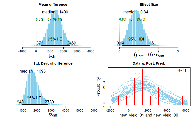
plot を使うと、事後分布を直接見ることができる。また、事後分布から抽出されたt分布が散在するヒストグラムの形で、事後予測チェックを得ることができる。モデルの適合度とデータの間に大きな不一致がある場合、先に進む前にもう一度考える必要がある。今のところ、post.pred.チェックは問題なさそうである。 　 この傾向も収量が増加しているが、推定値の精度は低く、95%信頼区間にはゼロが含まれる。また、新時代の国々と比べて、標準偏差が非常に大きいことも注目すべき点である。

fit <- bayes.t.test(new_yield_01, new_yield_80, paired = TRUE)
plot(fit)

summaryでは、事後分布の詳細な概要が表示される。この概要の小数点以下の桁数は、MCMCで近似しているため、実行ごとに数値が若干飛び交うことに注意。もしこれが気になるようであれば、bayes.t.testを呼び出す際に引数n.iterを使ってMCMCの反復回数を増やすとよいだろう。

summary(fit)

  Data
new_yield_01, n = 13
new_yield_80, n = 13

  Model parameters and generated quantities
mu_diff: the mean pairwise difference between new_yield_01 and new_yield_80 
sigma_diff: the scale of the pairwise difference, a consistent
  estimate of SD when nu is large.
nu: the degrees-of-freedom for the t distribution fitted to the pairwise difference
eff_size: the effect size calculated as (mu_diff - 0) / sigma_diff
diff_pred: predicted distribution for a new datapoint generated
  as the pairwise difference between new_yield_01 and new_yield_80 

  Measures
               mean       sd     HDIlo    HDIup %<comp %>comp
mu_diff    1405.128  525.778   375.531 2469.247  0.006  0.994
sigma_diff 1752.408  472.152   939.557 2739.324  0.000  1.000
nu           29.230   28.502     1.003   85.834  0.000  1.000
eff_size      0.855    0.365     0.143    1.565  0.006  0.994
diff_pred  1410.893 2474.509 -2882.521 5477.636  0.220  0.780

'HDIlo' and 'HDIup' are the limits of a 95% HDI credible interval.
'%<comp' and '%>comp' are the probabilities of the respective parameter being
smaller or larger than 0.

  Quantiles
               q2.5%     q25%   median     q75%   q97.5%
mu_diff      381.766 1068.847 1400.403 1732.760 2478.430
sigma_diff  1004.444 1432.091 1692.692 2000.098 2874.133
nu             2.293    9.439   20.266   39.476  106.273
eff_size       0.180    0.605    0.842    1.081    1.607
diff_pred  -2775.570  189.504 1400.464 2635.695 5612.202

diagnosticsは MCMC診断を表示し、プロットする（bayes.binom.testの例と同様）。最後にmodel.codeは、解析を再現する R と JAGS のコードを出力し、R スクリプトに直接コピー＆ペーストして、そこから変更することができる。さぁ、始めよう。

model.code(fit)

## Model code for Bayesian estimation supersedes the t test - paired samples ##
require(rjags)

# Setting up the data
x <- new_yield_01 
y <- new_yield_80 
pair_diff <- x - y
comp_mu <-  0 

# The model string written in the JAGS language
model_string <- "model {
  for(i in 1:length(pair_diff)) {
    pair_diff[i] ~ dt( mu_diff , tau_diff , nu )
  }
  diff_pred ~ dt( mu_diff , tau_diff , nu )
  eff_size <- (mu_diff - comp_mu) / sigma_diff
  
  mu_diff ~ dnorm( mean_mu , precision_mu )
  tau_diff <- 1/pow( sigma_diff , 2 )
  sigma_diff ~ dunif( sigma_low , sigma_high )
  # A trick to get an exponentially distributed prior on nu that starts at 1.
  nu <- nuMinusOne + 1 
  nuMinusOne ~ dexp(1/29)
}"

# Setting parameters for the priors that in practice will result
# in flat priors on mu and sigma.
mean_mu = mean(pair_diff, trim=0.2)
precision_mu = 1 / (mad(pair_diff)^2 * 1000000)
sigma_low = mad(pair_diff) / 1000 
sigma_high = mad(pair_diff) * 1000

# Initializing parameters to sensible starting values helps the convergence
# of the MCMC sampling. Here using robust estimates of the mean (trimmed)
# and standard deviation (MAD).
inits_list <- list(
  mu_diff = mean(pair_diff, trim=0.2),
  sigma_diff = mad(pair_diff),
  nuMinusOne = 4)

data_list <- list(
  pair_diff = pair_diff,
  comp_mu = comp_mu,
  mean_mu = mean_mu,
  precision_mu = precision_mu,
  sigma_low = sigma_low,
  sigma_high = sigma_high)

# The parameters to monitor.
params <- c("mu_diff", "sigma_diff", "nu", "eff_size", "diff_pred")

# Running the model
model <- jags.model(textConnection(model_string), data = data_list,
                    inits = inits_list, n.chains = 3, n.adapt=1000)
update(model, 500) # Burning some samples to the MCMC gods....
samples <- coda.samples(model, params, n.iter=10000)

# Inspecting the posterior
plot(samples)
summary(samples) 

例えば、ロバスト性はそれほど大きな問題ではなく、データがt分布ではなく正規分布であると仮定したい場合、このスクリプトを少し修正するだけでよい。モデルコードでは、dtをdnormに変更し、nuパラメータを削除し、このようなモデルになる。

model_string <- "model {
  for(i in 1:length(pair_diff)) {
    pair_diff[i] ~ dnorm( mu_diff , tau_diff)
  }
  diff_pred ~ dnorm( mu_diff , tau_diff)
  eff_size <- (mu_diff - comp_mu) / sigma_diff

  mu_diff ~ dnorm( mean_mu , precision_mu )
  tau_diff <- 1/pow( sigma_diff , 2 )
  sigma_diff ~ dunif( sigmaLow , sigmaHigh )
}"

またnuパラメータの監視を外す必要がある。

# The parameters to monitor.
params <- c("mu_diff", "sigma_diff", "eff_size", "diff_pred")

以上。