library(lavaan)
# HolzingerSwineford1939 データを読み込む
data(HolzingerSwineford1939)
head(HolzingerSwineford1939)
データはこのような感じ
  id sex ageyr agemo  school grade       x1   x2    x3       x4   x5        x6
1  1   1    13     1 Pasteur     7 3.333333 7.75 0.375 2.333333 5.75 1.2857143
2  2   2    13     7 Pasteur     7 5.333333 5.25 2.125 1.666667 3.00 1.2857143
3  3   2    13     1 Pasteur     7 4.500000 5.25 1.875 1.000000 1.75 0.4285714
4  4   1    13     2 Pasteur     7 5.333333 7.75 3.000 2.666667 4.50 2.4285714
5  5   2    12     2 Pasteur     7 4.833333 4.75 0.875 2.666667 4.00 2.5714286
6  6   2    14     1 Pasteur     7 5.333333 5.00 2.250 1.000000 3.00 0.8571429
        x7   x8       x9
1 3.391304 5.75 6.361111
2 3.782609 6.25 7.916667
3 3.260870 3.90 4.416667
4 3.000000 5.30 4.861111
5 3.695652 6.30 5.916667
6 4.347826 6.65 7.500000
とりあえず、schoolごとの平均点を計算してみよう。
library(dplyr)
HolzingerSwineford1939 %>%
  group_by(school) %>%
  summarise(across(x1:x9, mean))
school         x1    x2    x3    x4    x5    x6    x7    x8    x9
1 Grant-White  4.93  6.2   2.00  3.32  4.71  2.47  3.92  5.49  5.33
2 Pasteur      4.94  5.98  2.49  2.82  4.00  1.92  4.43  5.56  5.42
データの説明
- 被験者: 7歳から12歳の子供301人
- 検査: 知能検査
- 変数:
id: 被験者IDsex: 性別 (1 = 男性, 2 = 女性)ageyr: 年齢(年)agemo: 年齢(月)school: 学校名 (Pasteur, Grant-White)grade: 学年x1-x9: 知能検査の各項目の得点x1: Visual Perception (視覚的知覚)x2: Cubes (立方体)x3: Lozenges (菱形)x4: Paragraph Comprehension (段落理解)x5: Sentence Completion (文章完成)x6: Word Meaning (単語の意味)x7: Addition (加算)x8: Counting Dots (点の数え上げ)x9: Straight and Curved Capitals (直線と曲線の首都)
多母集団同時分析
# モデルを定義する
model.HS <- '
  visual =~ x1 + x2 + x3
  textual =~ x4 + x5 + x6
  speed =~ x7 + x8 + x9
'
# モデルをPasteur校とGrant-White校に同時に当てはめる
fit <- sem(model.HS,
           data = HolzingerSwineford1939,
           missing = "ML",
           group = "school",
           estimator = "MLR")

# 結果を表示
summary(fit, standardized = TRUE)
結果。
lavaan 0.6-19 ended normally after 60 iterations

  Estimator                                         ML
  Optimization method                           NLMINB
  Number of model parameters                        63
  Number of equality constraints                    15

  Number of observations per group:
    Pasteur                                        156
    Grant-White                                    145
  Number of missing patterns per group:
    Pasteur                                          1
    Grant-White                                      1

Model Test User Model:
                                              Standard      Scaled
  Test Statistic                               164.103     166.748
  Degrees of freedom                                60          60
  P-value (Chi-square)                           0.000       0.000
  Scaling correction factor                                  0.984
    Yuan-Bentler correction (Mplus variant)
  Test statistic for each group:
    Pasteur                                     91.665      91.665
    Grant-White                                 75.084      75.084

Parameter Estimates:

  Standard errors                             Sandwich
  Information bread                           Observed
  Observed information based on                Hessian


Group 1 [Pasteur]:

Latent Variables:
                   Estimate  Std.Err  z-value  P(>|z|)   Std.lv  Std.all
  visual =~
    x1                1.000                               0.892    0.768
    x2      (.p2.)    0.576    0.131    4.395    0.000    0.514    0.411
    x3      (.p3.)    0.798    0.173    4.627    0.000    0.712    0.591
  textual =~
    x4                1.000                               0.938    0.815
    x5      (.p5.)    1.120    0.067   16.623    0.000    1.050    0.829
    x6      (.p6.)    0.932    0.064   14.652    0.000    0.874    0.862
  speed =~
    x7                1.000                               0.568    0.516
    x8      (.p8.)    1.130    0.133    8.488    0.000    0.641    0.657
    x9      (.p9.)    1.009    0.207    4.864    0.000    0.573    0.578

Covariances:
                   Estimate  Std.Err  z-value  P(>|z|)   Std.lv  Std.all
  visual ~~
    textual           0.410    0.135    3.043    0.002    0.490    0.490
    speed             0.178    0.067    2.661    0.008    0.351    0.351
  textual ~~
    speed             0.180    0.062    2.889    0.004    0.338    0.338

Intercepts:
                   Estimate  Std.Err  z-value  P(>|z|)   Std.lv  Std.all
   .x1      (.25.)    5.001    0.094   53.050    0.000    5.001    4.302
   .x2      (.26.)    6.151    0.087   70.867    0.000    6.151    4.925
   .x3      (.27.)    2.271    0.095   24.016    0.000    2.271    1.885
   .x4      (.28.)    2.778    0.086   32.173    0.000    2.778    2.413
   .x5      (.29.)    4.035    0.103   39.095    0.000    4.035    3.184
   .x6      (.30.)    1.926    0.075   25.751    0.000    1.926    1.900
   .x7      (.31.)    4.242    0.079   53.702    0.000    4.242    3.855
   .x8      (.32.)    5.630    0.075   75.002    0.000    5.630    5.771
   .x9      (.33.)    5.465    0.072   76.114    0.000    5.465    5.516

Variances:
                   Estimate  Std.Err  z-value  P(>|z|)   Std.lv  Std.all
   .x1                0.555    0.184    3.017    0.003    0.555    0.411
   .x2                1.296    0.161    8.047    0.000    1.296    0.831
   .x3                0.944    0.147    6.446    0.000    0.944    0.650
   .x4                0.445    0.073    6.113    0.000    0.445    0.336
   .x5                0.502    0.081    6.197    0.000    0.502    0.313
   .x6                0.263    0.058    4.525    0.000    0.263    0.256
   .x7                0.888    0.128    6.952    0.000    0.888    0.734
   .x8                0.541    0.089    6.072    0.000    0.541    0.568
   .x9                0.654    0.115    5.685    0.000    0.654    0.666
    visual            0.796    0.239    3.336    0.001    1.000    1.000
    textual           0.879    0.135    6.513    0.000    1.000    1.000
    speed             0.322    0.092    3.499    0.000    1.000    1.000


Group 2 [Grant-White]:

Latent Variables:
                   Estimate  Std.Err  z-value  P(>|z|)   Std.lv  Std.all
  visual =~
    x1                1.000                               0.841    0.721
    x2      (.p2.)    0.576    0.131    4.395    0.000    0.484    0.442
    x3      (.p3.)    0.798    0.173    4.627    0.000    0.672    0.643
  textual =~
    x4                1.000                               0.933    0.847
    x5      (.p5.)    1.120    0.067   16.623    0.000    1.045    0.862
    x6      (.p6.)    0.932    0.064   14.652    0.000    0.869    0.796
  speed =~
    x7                1.000                               0.711    0.668
    x8      (.p8.)    1.130    0.133    8.488    0.000    0.803    0.773
    x9      (.p9.)    1.009    0.207    4.864    0.000    0.717    0.704

Covariances:
                   Estimate  Std.Err  z-value  P(>|z|)   Std.lv  Std.all
  visual ~~
    textual           0.427    0.107    4.003    0.000    0.544    0.544
    speed             0.329    0.101    3.268    0.001    0.550    0.550
  textual ~~
    speed             0.236    0.097    2.423    0.015    0.356    0.356

Intercepts:
                   Estimate  Std.Err  z-value  P(>|z|)   Std.lv  Std.all
   .x1      (.25.)    5.001    0.094   53.050    0.000    5.001    4.286
   .x2      (.26.)    6.151    0.087   70.867    0.000    6.151    5.618
   .x3      (.27.)    2.271    0.095   24.016    0.000    2.271    2.174
   .x4      (.28.)    2.778    0.086   32.173    0.000    2.778    2.522
   .x5      (.29.)    4.035    0.103   39.095    0.000    4.035    3.330
   .x6      (.30.)    1.926    0.075   25.751    0.000    1.926    1.763
   .x7      (.31.)    4.242    0.079   53.702    0.000    4.242    3.991
   .x8      (.32.)    5.630    0.075   75.002    0.000    5.630    5.422
   .x9      (.33.)    5.465    0.072   76.114    0.000    5.465    5.369
    visual           -0.148    0.140   -1.053    0.292   -0.176   -0.176
    textual           0.576    0.119    4.841    0.000    0.618    0.618
    speed            -0.177    0.104   -1.712    0.087   -0.250   -0.250

Variances:
                   Estimate  Std.Err  z-value  P(>|z|)   Std.lv  Std.all
   .x1                0.654    0.177    3.691    0.000    0.654    0.480
   .x2                0.964    0.152    6.351    0.000    0.964    0.804
   .x3                0.641    0.129    4.950    0.000    0.641    0.587
   .x4                0.343    0.065    5.275    0.000    0.343    0.283
   .x5                0.376    0.073    5.164    0.000    0.376    0.256
   .x6                0.437    0.074    5.922    0.000    0.437    0.366
   .x7                0.625    0.106    5.901    0.000    0.625    0.553
   .x8                0.434    0.147    2.948    0.003    0.434    0.403
   .x9                0.522    0.125    4.163    0.000    0.522    0.504
    visual            0.708    0.186    3.804    0.000    1.000    1.000
    textual           0.870    0.143    6.069    0.000    1.000    1.000
    speed             0.505    0.125    4.053    0.000    1.000    1.000
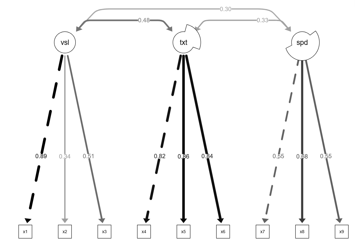
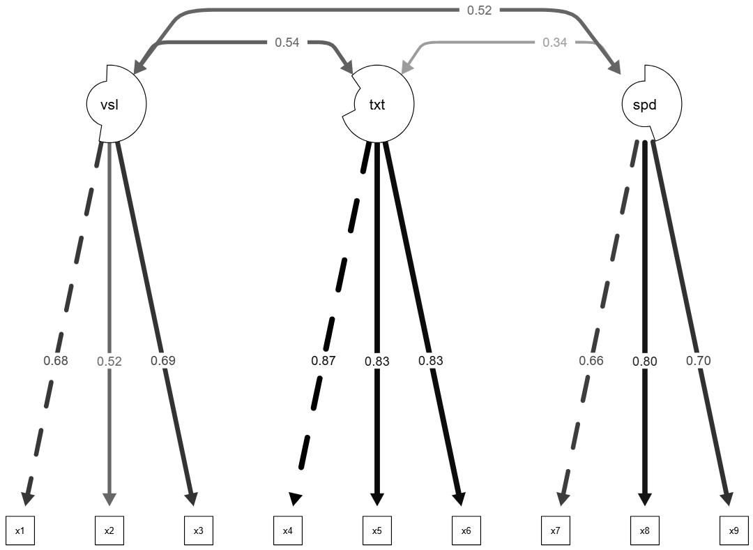
パス図
library(semPlot)
semPaths(fit,
         what = "std",
         layout = "tree2",
         curvePivot = TRUE,
         residuals = FALSE,
         intercepts = FALSE,
         edge.label.cex = 1.0,
         edge.color = "black",
         edge.label.position = 0.6,
         title = FALSE
         )