UCLA: Statistical Consulting Groupのページから。
UCLAではMplusのコードが書かれているが、このエントリでは、同じ分析をRのlavaanでの再現したいと思う。
Mplus
パス解析はすべての変数が観測される方程式系を推定するために使用される。潜在変数を含むモデルとは異なり、パス・モデルは,観察された変数の完全な測定を仮定する。観察された変数間の構造的関係のみがモデル化される。このタイプのモデルは、1つまたは複数の変数が他の2つの変数の関係を媒介すると考えられる場合によく使用されます(媒介モデル)。同様のモデル設定は、2つの無関係な従属変数の誤差(残差)が相関することが許されるモデル(一見無関連回帰)や、変数間の関係がグループ間で異なると考えられるモデル(多重グループモデル)の推定に使用することができる。
1.特定モデル
このページの例では、回答者の高校時代の成績 (hs), 大学時代の成績 (col), GRE のスコア (gre), そして大学院時代の成績 (grad) という 4 つの変数を含むデータセット (https://stats.idre.ucla.edu/wp-content/uploads/2016/02/path.dat) を使用している。GREスコアは高校と大学のGPA(それぞれhsとcol)を使って予測し、大学院のGPA(grad)はGRE、高校GPA、大学GPAを使って予測します。このモデルは、ちょうど同定され、自由度がゼロであることを意味する。
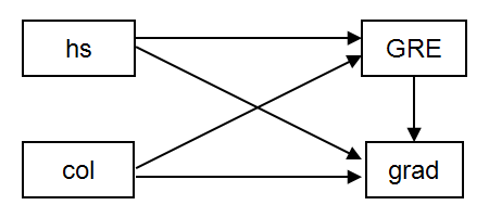
model: コマンドでは、on というキーワードで gre を hs と col に、grad を hs、col、gre に回帰させることを表しています。output: コマンドに stdyx; オプションをつけると、標準化された回帰係数とR2乗の値が得られる(stdyx; オプションは、回帰係数とR2乗の値が得られます)。(stdyx;オプションはyとxの両方で標準化された係数を生成するが、他のタイプの標準化も可能で、standardized;オプションを使って要求できる)。
Title: Path analysis -- just identified model
Data:
  file is https://stats.idre.ucla.edu/wp-content/uploads/2016/02/path.dat ;
Variable:
  Names are hs gre col grad;
Model:
    gre on hs col;
    grad on hs col gre;
Output:
    stdyx;
以下は、Mplusからの出力である。
INPUT READING TERMINATED NORMALLY


Path analysis -- just identified model

SUMMARY OF ANALYSIS

Number of groups                                                 1
Number of observations                                         200

Number of dependent variables                                    2
Number of independent variables                                  2
Number of continuous latent variables                            0

Observed dependent variables

  Continuous
   GRE         GRAD

Observed independent variables
   HS          COL


Estimator                                                       ML
Information matrix                                        OBSERVED
Maximum number of iterations                                  1000
Convergence criterion                                    0.500D-04
Maximum number of steepest descent iterations                   20

Input data file(s)
  https://stats.idre.ucla.edu/wp-content/uploads/2016/02/path.dat

Input data format  FREE


THE MODEL ESTIMATION TERMINATED NORMALLY


TESTS OF MODEL FIT

Chi-Square Test of Model Fit

          Value                              0.000
          Degrees of Freedom                     0
          P-Value                           0.0000

Chi-Square Test of Model Fit for the Baseline Model

          Value                            247.004
          Degrees of Freedom                     5
          P-Value                           0.0000

CFI/TLI

          CFI                                1.000
          TLI                                1.000

Loglikelihood

          H0 Value                       -2789.415
          H1 Value                       -2789.415

Information Criteria

          Number of Free Parameters              9
          Akaike (AIC)                    5596.830
          Bayesian (BIC)                  5626.515
          Sample-Size Adjusted BIC        5598.002
            (n* = (n + 2) / 24)

RMSEA (Root Mean Square Error Of Approximation)

          Estimate                           0.000
          90 Percent C.I.                    0.000  0.000
          Probability RMSEA <= .05           0.000

SRMR (Standardized Root Mean Square Residual)

          Value                              0.000


MODEL RESULTS

                                                    Two-Tailed
                    Estimate       S.E.  Est./S.E.    P-Value

 GRE      ON
    HS                 0.309      0.065      4.756      0.000
    COL                0.400      0.071      5.625      0.000

 GRAD     ON
    HS                 0.372      0.075      4.937      0.000
    COL                0.123      0.084      1.465      0.143
    GRE                0.369      0.078      4.754      0.000

 Intercepts
    GRE               15.534      2.995      5.186      0.000
    GRAD               6.971      3.506      1.989      0.047

 Residual Variances
    GRE               49.694      4.969     10.000      0.000
    GRAD              59.998      6.000     10.000      0.000


STANDARDIZED MODEL RESULTS


STDYX Standardization

                                                    Two-Tailed
                    Estimate       S.E.  Est./S.E.    P-Value

 GRE      ON
    HS                 0.335      0.068      4.887      0.000
    COL                0.396      0.068      5.859      0.000

 GRAD     ON
    HS                 0.356      0.070      5.073      0.000
    COL                0.108      0.073      1.467      0.142
    GRE                0.326      0.067      4.869      0.000

 Intercepts
    GRE                1.643      0.378      4.343      0.000
    GRAD               0.651      0.350      1.859      0.063

 Residual Variances
    GRE                0.556      0.052     10.611      0.000
    GRAD               0.523      0.051     10.240      0.000


R-SQUARE

    Observed                                        Two-Tailed
    Variable        Estimate       S.E.  Est./S.E.    P-Value

    GRE                0.444      0.052      8.477      0.000
    GRAD               0.477      0.051      9.333      0.000


QUALITY OF NUMERICAL RESULTS

     Condition Number for the Information Matrix              0.348E-04
       (ratio of smallest to largest eigenvalue)
MODEL RESULTS の下には、gre の hs と col への回帰のパス係数(スロープ)、そして grad の hs への回帰のパス係数が表示されています。標準化されていない係数(Estimateと書かれた列)と共に、標準誤差(S.E)、係数を標準誤差で割った値、そしてp値が示されている。ここから、hsとcolはgreを有意に予測し、greとhs(colは予測せず)はgradを有意に予測することがわかる。モデルからの追加パラメータは、パス係数の下に記載されている。これは、すべての係数(切片と傾き)が一緒に表示されるいくつかの汎用統計パッケージとは異なる。output: コマンドのstdyxオプションを使って標準化係数を要求したので、標準化結果も(非標準化結果の後に)出力に含まれます。STDYX標準化という見出しの下に、1単位の変化が元の変数の標準偏差の変化を表すように(標準化回帰モデルと同じように)標準化されたモデル・パラメータがすべてリストアップされている。標準化出力の一部として、R2乗の値がR-SQUAREの見出しの下に表示される。ここでは、我々のモデルの各従属変数の推定R2乗値が、標準誤差と仮説検定とともに与えられている。
2.間接効果および全体効果
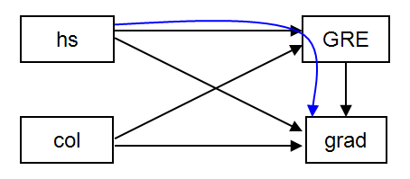
パスモデルの魅力の1つは,間接効果だけでなく,全体効果(すなわち,変数間の関係)を評価することができる点である.全体効果とは、直接効果と間接効果の組み合わせであることに注意。この例では、hsのgradへの間接効果の推定を求めます(greを通して)。下図は、このモデルに対応する図であり、希望する間接効果は青色で示されている。入力ファイルに model indirect: コマンドを追加し、grad ind hs; を指定することで、間接効果の推定値を得ることができる。
Title:  Path analysis -- with indirect effects.
Data:
  file is https://stats.idre.ucla.edu/wp-content/uploads/2016/02/path.dat ;
Variable:
  Names are hs gre col grad;
Model:
    gre on hs col;
    grad on hs col gre;
Model indirect:
    grad ind hs;
Output:
    stdyx;
このモデルの出力は以下のとおりである。このモデルの出力は、全体効果、間接効果、直接効果を示すセクションが追加されている以外は、前のモデルと同じなので、出力の一部を省略している。間接効果の追加により、Mplusから追加の出力が要求されるが、モデル自体は変わらないので、出力は同じです。合計、間接、および直接効果の内訳は、合計、合計間接、特殊間接、および直接効果とラベル付けされたセクションで、モデル結果と標準化モデル結果の下に表示される。標準化された係数が要求されたため、標準化された総効果、間接効果、直接効果が標準化されていない効果の下に表示されている。
MODEL RESULTS

                                                    Two-Tailed
                    Estimate       S.E.  Est./S.E.    P-Value

 GRE      ON
    HS                 0.309      0.065      4.756      0.000
    COL                0.400      0.071      5.625      0.000

 GRAD     ON
    HS                 0.372      0.075      4.937      0.000
    COL                0.123      0.084      1.465      0.143
    GRE                0.369      0.078      4.754      0.000

 Intercepts
    GRE               15.534      2.995      5.186      0.000
    GRAD               6.971      3.506      1.989      0.047

 Residual Variances
    GRE               49.694      4.969     10.000      0.000
    GRAD              59.998      6.000     10.000      0.000


<output omitted>

QUALITY OF NUMERICAL RESULTS

     Condition Number for the Information Matrix              0.348E-04
       (ratio of smallest to largest eigenvalue)


TOTAL, TOTAL INDIRECT, SPECIFIC INDIRECT, AND DIRECT EFFECTS


                                                    Two-Tailed
                    Estimate       S.E.  Est./S.E.    P-Value

Effects from HS to GRAD

  Total                0.487      0.075      6.453      0.000
  Total indirect       0.114      0.034      3.362      0.001

  Specific indirect

    GRAD
    GRE
    HS                 0.114      0.034      3.362      0.001

  Direct
    GRAD
    HS                 0.372      0.075      4.937      0.000


STANDARDIZED TOTAL, TOTAL INDIRECT, SPECIFIC INDIRECT, AND DIRECT EFFECTS


STDYX Standardization

                                                    Two-Tailed
                    Estimate       S.E.  Est./S.E.    P-Value

Effects from HS to GRAD

  Total                0.465      0.068      6.858      0.000
  Total indirect       0.109      0.032      3.455      0.001

  Specific indirect

    GRAD
    GRE
    HS                 0.109      0.032      3.455      0.001

  Direct
    GRAD
    HS                 0.356      0.070      5.073      0.000
具体的な間接効果では、GRAD GRE HS と書かれた効果(それぞれが独立した行に表示され、最終結果が最初に表示されることに注意)は、GRE(上の青いパス)を通じて、新卒に対する HS の間接効果に対する推定係数を示している。直接効果と書かれた係数は、hsが学位に与える直接的な効果である。しかし、hsからgradへの有意な直接経路は、部分的な仲介に過ぎないことを示唆している。
3.具体的な間接効果
上記の例では、間接効果が1つしかないため、単純に過ぎた。多くの場合、モデルには複数の間接効果がある。この例では、hsからcolへの方向性パス(つまり回帰)を配置し、複数の間接効果の可能性があるモデルを作成する。下の図は、モデルを示しており、検討したい3つの間接パスを色付きの線で強調している。
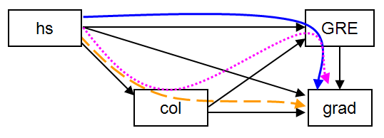
間接効果の計算を要求する方法はいくつかある。最初の方法は、前の例で示したもの(すなわち、grad ind hs;)で、hs から grad までのすべての間接パスを要求するものである。また、indを使って特定の間接パスを要求することもできます。例えば、以下ではgrad ind col hs;を使って、hs→col→gradの間接効果(つまり、上図のオレンジの破線のパス)を推定したいことを指定している。最後に、via を使って、第3の変数を通るすべての間接効果を要求できる。例えば、以下では、grad via gre hs; を使って、hs から grad へのすべての間接パスで gre を含むものを要求する。これは、hs から gre から grad(つまり、青の実線のパス)、hs から col から gre から grad(つまり、ピンクの点線のパス)である。新しい方向パス (col on hs;) と、モデル間接の特定の間接 (grad ind col hs;) と経由 (grad via gre hs;) オプションは、下図の入力で強調表示されている。
Title: Multiple indirect paths
Data:
  file is https://stats.idre.ucla.edu/wp-content/uploads/2016/02/path.dat ;
Variable:
  Names are hs gre col grad;
Model:
  gre on col hs;
  grad on hs col gre;
  col on hs;
Model indirect:
  grad ind col hs;
  grad via gre hs;
簡略化した出力は以下。このモデルの出力は、間接効果を示すセクションが追加されている以外は、以前のモデルの出力と同様の構造であることに注意。
<output omitted>

TOTAL, TOTAL INDIRECT, SPECIFIC INDIRECT, AND DIRECT EFFECTS


                                                    Two-Tailed
                    Estimate       S.E.  Est./S.E.    P-Value

Effects from HS to GRAD

  Sum of indirect      0.075      0.051      1.455      0.146

  Specific indirect

    GRAD
    COL
    HS                 0.075      0.051      1.455      0.146


Effects from HS to GRAD via GRE

  Sum of indirect      0.204      0.047      4.333      0.000

  Specific indirect
    GRAD
    GRE
    HS                 0.114      0.034      3.362      0.001

    GRAD
    GRE
    COL
    HS                 0.090      0.026      3.487      0.000
間接効果の最初のセット(HSからGRADへの効果)では、hs の col を通じた grad に対する間接効果が示されている。このモデルでは、hsのgradへの直接効果を推定したが、特定の間接効果を求めたため、この部分には表示されていない(上に表示されている)。間接効果の2番目のセット(HSからGREを経由したGRADへの効果)は、GREを含むhsからgradへのすべての間接効果(この場合、2つの間接効果がある)を示している。この出力は、hsがgradに対して全体として有意な間接効果(間接効果の和)を持ち、さらに2つの特定の間接効果(gre経由、colとgre経由)を持っていることを示している。この出力は、hsに対するgradの全効果を含んでいないことに注意。この出力では、前のモデルで行ったように、grad ind hsと指定するだけである。
過剰同定モデル
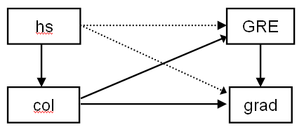
これは過剰同定モデルの例で、正の自由度を持つモデルである(飽和または単に同定されたと表現できる以前のモデルとは対照的である)。正の自由度を持つことで、CFIやRMSEAなどの適合指標とともに、モデル適合のカイ2乗検定を使用して、モデルの適合性を調査することができる。下の図では、モデルに含まれるパスは実線で表され、推定できるがそうでないパスは点線で表されている。hsはgradにもgreにも直接的な影響を与えず、colを経由してのみ影響を与えることに注意されたい。これは、高校の GPA は大学の GPA との関係を通してのみ、GRE の得点や大学院の成績と関連する、という仮説に対応するものである。
Title: Path analysis -- over identified model
Data:
  file is https://stats.idre.ucla.edu/wp-content/uploads/2016/02/path.dat ;
Variable:
  Names are hs gre col grad;
Model:
  col on hs;
  gre on col;
  grad on col gre;
Output:
  stdyx;
結果。
INPUT READING TERMINATED NORMALLY

Path analysis -- over identified model

SUMMARY OF ANALYSIS

Number of groups                                                 1
Number of observations                                         200

Number of dependent variables                                    3
Number of independent variables                                  1
Number of continuous latent variables                            0

Observed dependent variables

  Continuous
   GRE         COL         GRAD

Observed independent variables
   HS


Estimator                                                       ML
Information matrix                                        OBSERVED
Maximum number of iterations                                  1000
Convergence criterion                                    0.500D-04
Maximum number of steepest descent iterations                   20

Input data file(s)
  https://stats.idre.ucla.edu/wp-content/uploads/2016/02/path.dat

Input data format  FREE


THE MODEL ESTIMATION TERMINATED NORMALLY


TESTS OF MODEL FIT

Chi-Square Test of Model Fit

          Value                             44.429
          Degrees of Freedom                     2
          P-Value                           0.0000

Chi-Square Test of Model Fit for the Baseline Model

          Value                            362.474
          Degrees of Freedom                     6
          P-Value                           0.0000

CFI/TLI

          CFI                                0.881
          TLI                                0.643

Loglikelihood

          H0 Value                       -2811.629
          H1 Value                       -2789.415

Information Criteria

          Number of Free Parameters             10
          Akaike (AIC)                    5643.258
          Bayesian (BIC)                  5676.242
          Sample-Size Adjusted BIC        5644.561
            (n* = (n + 2) / 24)

RMSEA (Root Mean Square Error Of Approximation)

          Estimate                           0.3266
          90 Percent C.I.                    0.247  0.412
          Probability RMSEA <= .05           0.000

SRMR (Standardized Root Mean Square Residual)

          Value                              0.086


MODEL RESULTS

                                                    Two-Tailed
                    Estimate       S.E.  Est./S.E.    P-Value

 COL      ON
    HS                 0.605      0.048     12.500      0.000

 GRE      ON
    COL                0.625      0.056     11.101      0.000

 GRAD     ON
    COL                0.317      0.079      4.014      0.000
    GRE                0.492      0.078      6.303      0.000

 Intercepts
    GRE               19.887      3.009      6.609      0.000
    COL               21.038      2.576      8.165      0.000
    GRAD               9.779      3.664      2.669      0.008

 Residual Variances
    GRE               55.313      5.531     10.000      0.000
    COL               49.025      4.903     10.000      0.000
    GRAD              67.311      6.731     10.000      0.000


STANDARDIZED MODEL RESULTS


STDYX Standardization

                                                    Two-Tailed
                    Estimate       S.E.  Est./S.E.    P-Value

 COL      ON
    HS                 0.662      0.040     16.684      0.000

 GRE      ON
    COL                0.617      0.044     14.112      0.000

 GRAD     ON
    COL                0.276      0.068      4.092      0.000
    GRE                0.434      0.065      6.671      0.000

 Intercepts
    GRE                2.103      0.397      5.298      0.000
    COL                2.251      0.363      6.210      0.000
    GRAD               0.913      0.375      2.436      0.015

 Residual Variances
    GRE                0.619      0.054     11.452      0.000
    COL                0.561      0.053     10.677      0.000
    GRAD               0.587      0.053     11.002      0.000


R-SQUARE

    Observed                                        Two-Tailed
    Variable        Estimate       S.E.  Est./S.E.    P-Value

    GRE                0.381      0.054      7.056      0.000
    COL                0.439      0.053      8.342      0.000
    GRAD               0.413      0.053      7.743      0.000


QUALITY OF NUMERICAL RESULTS

     Condition Number for the Information Matrix              0.104E-03
       (ratio of smallest to largest eigenvalue)
カイ二乗の値は、現在のモデルと飽和したモデルを比較する。我々のモデルは飽和していない(すなわち、我々のモデルは正の自由度を持つ)ので、カイ2乗値はもはやゼロではなく、モデルの適合性を評価するために使用することができる。同様に、同定されたばかりのモデルで1に等しかったCFIとTLIは、現在、情報量を持つ値になっている。さらに、RMSEAとSRMRは、情報量の多い値をとるようになりました(同定されたばかりのモデルでは、それらはゼロとして表示される)。正の自由度を持ち、したがって適合度指標に有益な値を持つことで、我々のモデルがどの程度データに適合しているかをよりよく評価することができる。このモデルからの具体的な係数推定値は、一般に、同定されたばかりのモデルと同じように解釈される。
R
データ読み込み
df1 <- read.table('https://stats.idre.ucla.edu/wp-content/uploads/2016/02/path.dat', sep=",")
colnames(df1)<-c("hs","gre","col","grad")
1.特定モデル
library(lavaan)
model1 <- '
  gre ~ hs
  gre ~ col
  grad ~  hs
  grad ~  col
  grad ~  gre
'
fit1 <- sem(model = model1, data=df1)
summary(fit1, standardized=TRUE)
結果。
Regressions:
                   Estimate  Std.Err  z-value  P(>|z|)   Std.lv  Std.all
  gre ~
    hs                0.309    0.065    4.756    0.000    0.309    0.335
    col               0.400    0.071    5.626    0.000    0.400    0.396
  grad ~
    hs                0.372    0.075    4.937    0.000    0.372    0.356
    col               0.123    0.084    1.465    0.143    0.123    0.108
    gre               0.369    0.078    4.755    0.000    0.369    0.326

Variances:
                   Estimate  Std.Err  z-value  P(>|z|)   Std.lv  Std.all
   .gre              49.694    4.969   10.000    0.000   49.694    0.556
   .grad             59.998    6.000   10.000    0.000   59.998    0.523
2.間接効果および全体効果
model2 <- '
# direct effect
  grad ~ c*hs

# mediator
  gre ~ a*hs
  grad ~ b*gre

# indirect effect (a*b)
  ab := a*b

# total effect
  total := c + (a*b)

# another path
  gre ~ col
  grad ~  col
'
ラベルをそれぞれにつける。
独立変数Xにはc
従属変数Yにはb
媒介変数Mにはa
ラベルは任意でよい。間接効果の書き方は以下。
まず:=は母数を定義づけるための記号である。
abはa*bと定義づけられている。ここが間接効果に相当する。間接効果は構成する2つのパスの積であるため定義が積になっている。\
totalというのは総合効果であり、c + (a*b)と定義づけられる。ちなみにcは直接効果である。
fit2 <- sem(model = model2, data=df1)
summary(fit2, standardized=TRUE)
3.具体的な間接効果
model3 <- '
# direct effect
  grad ~ c*hs

# mediator
  gre ~ a*hs
  grad ~ b*gre
  gre ~ f*col
  col ~ d*hs
  grad ~ e*col


# indirect effect
  ab := a*b # hs -> tre -> grad
  dfb := d*f*b # hs -> col -> gre -> grad
  de := d*e # hs -> col -> grad

# total effect
  total_ind := (a*b) + (d*f*b)
'
fit3 <- sem(model = model3, data=df1)
summary(fit3, standardized=TRUE)
結果。
Regressions:
                   Estimate  Std.Err  z-value  P(>|z|)   Std.lv  Std.all
  grad ~
    hs         (c)    0.372    0.075    4.937    0.000    0.372    0.356
  gre ~
    hs         (a)    0.309    0.065    4.756    0.000    0.309    0.335
  grad ~
    gre        (b)    0.369    0.078    4.755    0.000    0.369    0.326
  gre ~
    col        (f)    0.400    0.071    5.626    0.000    0.400    0.396
  col ~
    hs         (d)    0.605    0.048   12.500    0.000    0.605    0.662
  grad ~
    col        (e)    0.123    0.084    1.465    0.143    0.123    0.108

Variances:
                   Estimate  Std.Err  z-value  P(>|z|)   Std.lv  Std.all
   .grad             59.998    6.000   10.000    0.000   59.998    0.523
   .gre              49.694    4.969   10.000    0.000   49.694    0.556
   .col              49.025    4.903   10.000    0.000   49.025    0.561

Defined Parameters:
                   Estimate  Std.Err  z-value  P(>|z|)   Std.lv  Std.all
    ab                0.114    0.034    3.362    0.001    0.114    0.109
    dfb               0.090    0.026    3.487    0.000    0.090    0.086
    de                0.075    0.051    1.455    0.146    0.075    0.071
    total_ind         0.204    0.047    4.332    0.000    0.204    0.195
hs -> tre -> grad: ab = 0.114
hs -> col -> gre -> grad : dfb = 0.090
hs -> col -> grad : de = 0.075
Effects from HS to GRAD via GRE
Sum of indirect : ab + dfb = 0.204
4.過剰同定モデル
model4 <- '
  col ~ hs
  gre ~ col
  grad ~ col
  grad ~ gre
'
fit4 <- sem(model = model4, data=df1)
summary(fit4, standardized=TRUE, fit.measures=TRUE) #フィット指標の表示
結果。
  Estimator                                         ML
  Optimization method                           NLMINB
  Number of model parameters                         7

  Number of observations                           200

Model Test User Model:

  Test statistic                                44.429
  Degrees of freedom                                 2
  P-value (Chi-square)                           0.000

Model Test Baseline Model:

  Test statistic                               362.474
  Degrees of freedom                                 6
  P-value                                        0.000

User Model versus Baseline Model:

  Comparative Fit Index (CFI)                    0.881
  Tucker-Lewis Index (TLI)                       0.643

Loglikelihood and Information Criteria:

  Loglikelihood user model (H0)              -2062.830
  Loglikelihood unrestricted model (H1)      -2040.616

  Akaike (AIC)                                4139.660
  Bayesian (BIC)                              4162.748
  Sample-size adjusted Bayesian (BIC)         4140.571

Root Mean Square Error of Approximation:

  RMSEA                                          0.326
  90 Percent confidence interval - lower         0.247
  90 Percent confidence interval - upper         0.412
  P-value RMSEA <= 0.05                          0.000

Standardized Root Mean Square Residual:

  SRMR                                           0.102

Parameter Estimates:

  Standard errors                             Standard
  Information                                 Expected
  Information saturated (h1) model          Structured

Regressions:
                   Estimate  Std.Err  z-value  P(>|z|)   Std.lv  Std.all
  col ~
    hs                0.605    0.048   12.500    0.000    0.605    0.662
  gre ~
    col               0.625    0.056   11.101    0.000    0.625    0.617
  grad ~
    col               0.317    0.079    4.014    0.000    0.317    0.276
    gre               0.492    0.078    6.303    0.000    0.492    0.434

Variances:
                   Estimate  Std.Err  z-value  P(>|z|)   Std.lv  Std.all
   .col              49.025    4.903   10.000    0.000   49.025    0.561
   .gre              55.313    5.531   10.000    0.000   55.313    0.619
   .grad             67.311    6.731   10.000    0.000   67.311    0.587