ブートストラップは、サンプルからの統計量を推定するために、置換を伴うランダム・サンプリングを使用する。このサンプルからリサンプリングを行うことで、母集団を代表するような新しいデータを生成することができる。小さな標本から1度だけ統計量を推定する代わりに、統計量を複数回推定することができます。したがって、10回リサンプリングすれば、目的の統計量の推定値を10回計算することになる。
ブートストラップの手順は次のとおりである:
- データをn回置換してリサンプリングする
- 目的の統計量をn回計算して、推定統計量の分布を生成する
- ブートストラップされた分布から、ブートストラップされた統計量の標準誤差/信頼区間を決定する
この記事では、TidyTuesdayの過去の学費データセットを使って、私立大学と公立大学の学費の関係を推定するためにブートストラップリサンプリングを行う方法を紹介する。
はじめに、GitHubからデータを読み込む。
library(tidyverse)
library(tidymodels)
historical_tuition <- readr::read_csv('https://raw.githubusercontent.com/rfordatascience/tidytuesday/master/data/2020/2020-03-10/historical_tuition.csv')
head(historical_tuition)
# A tibble: 6 x 4
  type             year    tuition_type    tuition_cost
  <chr>            <chr>   <chr>                  <dbl>
1 All Institutions 1985-86 All Constant           10893
2 All Institutions 1985-86 4 Year Constant        12274
3 All Institutions 1985-86 2 Year Constant         7508
4 All Institutions 1985-86 All Current             4885
5 All Institutions 1985-86 4 Year Current          5504
6 All Institutions 1985-86 2 Year Current          3367
現在、データは各行が1つのオブザベーションを表すロングフォーマットである。各年度に複数のオブザベーションがあり、各機関タイプからのデータを表している: 公立、私立、全教育機関。リサンプリングでデータを利用するためには、私立学校の授業料を含む1つの列と公立学校の授業料を含むもう1つの列を持つワイド・フォーマットにデータを変換する必要がある。このワイドフォーマットの各行は、特定の年の過去の授業料を表す。以下は、ロングフォーマットのデータをワイドフォーマットに変換するコードである。モデル化するために注目する列は、year 列で指定された特定の年度の公立学校と私立学校の授業料を表す public と private である。
tuition_df <- historical_tuition %>%
  pivot_wider(names_from = type,
              values_from = tuition_cost
              ) %>%
  na.omit() %>%
  janitor::clean_names()
データ。
# A tibble: 25 x 5
   year    tuition_type    all_institutions public private
   <chr>   <chr>                      <dbl>  <dbl>   <dbl>
 1 1985-86 All Constant               10893   7964   19812
 2 1985-86 4 Year Constant            12274   8604   20578
 3 1985-86 2 Year Constant             7508   6647   14521
 4 1985-86 All Current                 4885   3571    8885
 5 1985-86 4 Year Current              5504   3859    9228
 6 1985-86 2 Year Current              3367   2981    6512
 7 1995-96 All Constant               13822   9825   27027
 8 1995-96 4 Year Constant            16224  11016   27661
 9 1995-96 2 Year Constant             7421   6623   18161
10 1995-96 All Current                 8800   6256   17208
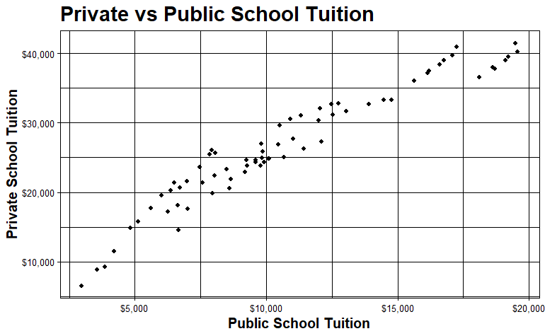
私立と公立の学費の関係を視覚化することができる。
tuition_df %>%
  ggplot(aes(public, private))+
  geom_point()+
  scale_y_continuous(labels=scales::dollar_format())+
  scale_x_continuous(labels=scales::dollar_format())+
  ggtitle("Private vs Public School Tuition")+
  xlab("Public School Tuition")+
  ylab("Private School Tuition")+
  theme_linedraw()+
  theme(axis.title=element_text(size=14,face="bold"),
        plot.title = element_text(size = 20, face = "bold"))
私立校と公立校の授業料には直接的な正の関係があるようだ。一般的に、私立学校の学費は公立学校よりも高い。私立学校の方が公立学校よりも学費が高い。
私立学校と公立学校の学費の関係を調べるために、データに線形フィットを行うことができる。Rのlm関数でこれを行うことができる。傾きは2.38と推定されることがわかる。公立学校の授業料1ドルに対して、私立学校の授業料は約2.38倍となる。
tuition_fit <- lm(private ~ 0 + public,
               data = tuition_df)
summary(tuition_fit)
結果。
Coefficients:
       Estimate Std. Error t value Pr(>|t|)
public   2.3790     0.0346   68.75   <2e-16 ***
次に、リサンプリングを使って、公立学校と私立学校の学費の関係をより正確に推定することを試みる。ブートストラップでは、元のデータセットから、元のデータセットと同じサイズの新しいデータセットを作成するために、置換を伴う無作為抽出を行う。これは本質的に、元のデータセットから新しいデータセットを生成するシミュレーションである。データを1,000回リサンプリングする。
## set.seedに乱数列を生成するための開始番号を設定し、再現可能な結果を得られるようにする。
set.seed(123)
tution_boot <- bootstraps(tuition_df,
                          times = 1e3,
                          apparent = TRUE)
次に、1,000回の再標本化に線形モデルをあてはめる。これらの結果は model という新しいカラムに格納され、統計量は conf_infというカラムに格納される。そして、推定統計量(直線の傾き)、誤差、p値を抽出するために、結果をアンネストする。
tuition_models <- tution_boot %>%
  mutate(model = map(splits, ~lm(private ~ 0 + public,
               data = .) ),
         coef_inf = map(model, tidy))
tuition_coefs <- tuition_models %>%
  unnest(coef_inf)
lmの結果。
   splits          id            model  term   estimate std.error statistic  p.value
   <list>          <chr>         <list> <chr>     <dbl>     <dbl>     <dbl>    <dbl>
 1 <split [72/30]> Bootstrap0001 <lm>   public     2.45    0.0335      73.3 1.24e-68
 2 <split [72/26]> Bootstrap0002 <lm>   public     2.42    0.0364      66.6 9.95e-66
 3 <split [72/29]> Bootstrap0003 <lm>   public     2.43    0.0331      73.5 9.62e-69
 4 <split [72/26]> Bootstrap0004 <lm>   public     2.45    0.0400      61.2 3.37e-63
 5 <split [72/24]> Bootstrap0005 <lm>   public     2.37    0.0328      72.3 2.98e-68
 6 <split [72/21]> Bootstrap0006 <lm>   public     2.34    0.0345      67.8 2.86e-66
 7 <split [72/26]> Bootstrap0007 <lm>   public     2.37    0.0328      72.2 3.46e-68
 8 <split [72/22]> Bootstrap0008 <lm>   public     2.33    0.0355      65.6 2.73e-65
 9 <split [72/25]> Bootstrap0009 <lm>   public     2.42    0.0332      72.8 1.98e-68
10 <split [72/26]> Bootstrap0010 <lm>   public     2.42    0.0331      73.0 1.64e-68
今、私立学校と公立学校の授業料の関係について、リサンプリングから得られた1,000の推定値があり、estimate列に格納されている。ここで、私立学校と公立学校の授業料の間の推定された傾きの分布はどのようなものかという疑問が生じる。
tuition_coefs %>%
  ggplot(aes(estimate))+
  geom_histogram(alpha = .7)+
  ggtitle("Distribution of Estimated Slope")+
  xlab("Estimate")+
  ylab("Frequency")+
  theme_linedraw()+
  theme(axis.title=element_text(size=14,face="bold"),
        plot.title = element_text(size = 20, face = "bold"))

int_pctl(tuition_models,
         coef_inf)
  term   .lower .estimate .upper .alpha .method
  <chr>   <dbl>     <dbl>  <dbl>  <dbl> <chr>
1 public   2.31      2.38   2.46   0.05 percentile
ブートストラップにより、私立学校と公立学校の学費の関係を表す推定勾配は約2.38であり、ブートストラップなしで得られたものと同様であることがわかる。これは、公立学校と私立学校の間の基本的な関係が線形であり、線形モデルの基本的な仮定がこのデータセットに適用されるためと考えられます。線形回帰の基本的な仮定は以下の通りである:
- 変数間の基本的関係は線形である。
- 誤差が正規分布している
- ベスト・フィットの線の周りに等しい分散がある(誤差の同相分散性)
- 観測値が独立である
さらに、ブートストラップでは、未サンプルのデータに対して線形モデルを使用しただけでは得られなかった、関係の下界と上界を得ることができる。
最後に、ブートストラップしたサンプルから計算した様々な推定値を可視化することができる。
tuition_aug <- tuition_models %>%
  # Sample only 200 bootstraps for visualization
  sample_n(200) %>%
  mutate(augmented = map(model, augment)) %>%
  unnest(augmented)
tuition_aug %>%
  ggplot(aes(public, private))+
  geom_line(aes(y = .fitted, group = id), alpha = .1, color = 'grey')+
  geom_point()+
  scale_y_continuous(labels=scales::dollar_format())+
  scale_x_continuous(labels=scales::dollar_format())+
  ggtitle("200 of 1000 Slope Estimations from Bootstrap Resampling")+
  xlab("Public School Tuition")+
  ylab("Private School Tuition")+
  theme_linedraw()+
  theme(axis.title=element_text(size=14,face="bold"),
        plot.title = element_text(size = 20, face = "bold"))

要約すると、このブログでは、私立学校と公立学校の授業料の関係を決定するためにRでブートストラップ・リスンプリングを使用する方法を示した。この手法は、ランダム・サンプリングを使って、ほぼすべての統計量のサンプリング分布を推定する。