データの準備
library(haven)
library(tidyr)
auto_data <- haven::read_dta("http://www.stata-press.com/data/r9/auto.dta")
auto_data <- auto_data %>% drop_na()  # 全カラムに対してNAがない行を抽出
auto_data$foreign <- as.integer(auto_data$foreign)

price_data <- auto_data$price
X_data <- auto_data[, c("mpg", "rep78", "headroom", "trunk", "weight", "length",
                        "turn", "displacement", "gear_ratio", "foreign")]
X_data <- as.matrix(X_data)
安定性選択の実行
stabsel関数を使用する際に、特に次の3つの仮定(assumption)を指定する。
- Unimodal: この仮定は、選択確率の分布が一峰性であると仮定する。つまり、選択確率が一つの山(モード)を持つ分布に従うことを前提とする。通常、選択確率が高い変数は、信頼性の高い変数とみなされる。
- R-concave: この仮定は、選択確率の分布がr凹性であることを仮定する。これは、選択確率の分布が特定の凹状の形状を持つことを前提としている。R-concave仮定を使用することで、選択確率の分布がより一般的な形状を持つ場合にも適用可能である。
- None: この仮定は、選択確率の分布に特定の形状を仮定しないことを意味する。つまり、分布がどのような形状であっても受け入れられる。この設定は、特にサンプリングタイプがMB(Meinshausen & Buehlmann, 2010)の場合に使用される。
ここではsampling.type = "SS"を使用する。SSは下記の論文での方法論である。
- R.D. Shah and R.J. Samworth (2013), Variable selection with error control: another look at stability selection. Journal of the Royal Statistical Society, Series B, 75, 55--80.
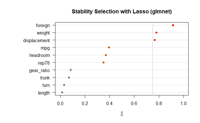
library(glmnet)
library(stabs)
library(dplyr)

set.seed(123)  # 再現性のためのシード設定
# 安定性選択の実行
stab_glmnet_model <- stabsel(
  x = X_data,
  y = price_data,
  fitfun = glmnet.lasso,
  cutoff = 0.75,
  PFER = 1,
  B = 100,
  sampling.type = "SS",
  assumption = "r-concave"
)

# 結果の表示
print(stab_glmnet_model)
plot(stab_glmnet_model, main = "Stability Selection with Lasso (glmnet)")
 Stability Selection with r-concavity assumption

Selected variables:
      weight displacement      foreign
           5            8           10

Selection probabilities:
      length         turn        trunk   gear_ratio        rep78     headroom          mpg displacement       weight      foreign
       0.015        0.030        0.070        0.085        0.350        0.370        0.395        0.765        0.780        0.915

---
Cutoff: 0.75; q: 4; PFER (*):  0.845
   (*) or expected number of low selection probability variables
PFER (specified upper bound):  1
PFER corresponds to signif. level 0.0845 (without multiplicity adjustment)
Lasso回帰とRidge回帰を用いて推定
selected_indices <- stab_glmnet_model$selected
selected_variables <- colnames(X_data)[selected_indices]

if (length(selected_variables) == 0) {
  print("選ばれた変数がありません。")
} else {
  X_selected_data <- X_data[, selected_variables, drop = FALSE]

  if (ncol(X_selected_data) == 1) {
    X_selected_data <- as.matrix(X_selected_data)
    colnames(X_selected_data) <- selected_variables
  }

  # Lasso回帰
  lasso_cv_model <- cv.glmnet(X_selected_data, price_data, alpha = 1)
  best_lambda_lasso <- lasso_cv_model$lambda.min
  lasso_coefficients <- coef(lasso_cv_model, s = best_lambda_lasso)
  print("Lasso回帰の結果:")
  print(paste("Best Lambda: ", best_lambda_lasso))
    print(lasso_coefficients)

  # Ridge回帰
  ridge_cv_model <- cv.glmnet(X_selected_data, price_data, alpha = 0)
  best_lambda_ridge <- ridge_cv_model$lambda.min
  ridge_coefficients <- coef(ridge_cv_model, s = best_lambda_ridge)
    print("Ridge回帰の結果:")
  print(paste("Best Lambda: ", best_lambda_ridge))
  print(ridge_coefficients)
}
[1] "Lasso回帰の結果:"
[1] "Best Lambda:  5.96437147505912"
4 x 1 sparse Matrix of class "dgCMatrix"
                       s1
(Intercept)  -3520.061513
weight           1.894351
displacement    14.016316
foreign       3769.198043

[1] "Ridge回帰の結果:"
[1] "Best Lambda:  158.418942078602"
4 x 1 sparse Matrix of class "dgCMatrix"
                       s1
(Intercept)  -2677.702583
weight           1.701122
displacement    13.424760
foreign       3311.321977
ブートストラップを使ったRidge回帰での推定
各ブートストラップサンプルに対してモデルを構築し、その結果を集計することで、推定値の安定性を高められる。
X_selected_data <- X_data[, selected_variables, drop = FALSE]

if (ncol(X_selected_data) == 1) {
    X_selected_data <- as.matrix(X_selected_data)
    colnames(X_selected_data) <- selected_variables
}

# ブートストラップ法を用いて安定した推定値を計算
set.seed(123)
n_bootstrap <- 1000
bootstrap_coefficients <- matrix(NA, ncol = ncol(X_selected_data) + 1, nrow = n_bootstrap) # +1 for intercept

for (i in 1:n_bootstrap) {
  set.seed(i)
  bootstrap_indices <- sample(1:nrow(X_selected_data), replace = TRUE)
  X_bootstrap <- X_selected_data[bootstrap_indices, ]
  y_bootstrap <- price_data[bootstrap_indices]

  ridge_model_bootstrap <- glmnet(X_bootstrap, y_bootstrap, alpha = 0)
  cv_ridge_model_bootstrap <- cv.glmnet(X_bootstrap, y_bootstrap, alpha = 0)
  best_lambda_ridge_bootstrap <- cv_ridge_model_bootstrap$lambda.min
  ridge_coefficients_bootstrap <- coef(ridge_model_bootstrap, s = best_lambda_ridge_bootstrap)

  bootstrap_coefficients[i, ] <- as.vector(ridge_coefficients_bootstrap)
}

# 推定値の平均と標準偏差を計算
mean_coefficients <- colMeans(bootstrap_coefficients, na.rm = TRUE)
sd_coefficients <- apply(bootstrap_coefficients, 2, sd, na.rm = TRUE)

# 結果の表示
results_bootstrap <- data.frame(
  Variable = c("(Intercept)", selected_variables),
  Mean = mean_coefficients,
  SD = sd_coefficients
)

print(results_bootstrap)
      Variable         Mean           SD
1  (Intercept) -2703.937195 1387.1918186
2       weight     1.733702    0.5080322
3 displacement    12.966528    4.5688871
4      foreign  3299.952422  616.2677086
# 必要なライブラリの読み込み
library(ggplot2)

# グラフの作成
ggplot(results_bootstrap, aes(x = Variable, y = Mean)) +
  geom_bar(stat = "identity", fill = "skyblue", width = 0.5) +
  geom_errorbar(aes(ymin = Mean - SD, ymax = Mean + SD), width = 0.2, color = "blue") +
  labs(title = "Mean and Standard Deviation of Coefficients",
       x = "Variable",
       y = "Value") +
  theme_minimal()

異なる乱数シードを用いた反復計算
# 選ばれた変数のみを用いて新たにモデルを再構築
X_selected <- X_data[, selected_vars, drop = FALSE]

if (ncol(X_selected) == 1) {
  X_selected <- as.matrix(X_selected)
  colnames(X_selected) <- selected_vars
}
# 並列処理の設定
num_cores <- detectCores() - 2  # システム全体のコア数から2つを引いた数を使用
cl <- makeCluster(num_cores)
registerDoParallel(cl)

# 結果を格納するリストを初期化
coef_list <- list()
n_repeats <- 1000

# 1000回の反復計算
for (i in 1:n_repeats) {
  set.seed(i)  # 異なる乱数シードを設定

  # リッジ回帰のモデルの作成
  final_model <- glmnet(X_selected, price_data, alpha = 0)
  cv_final_model <- cv.glmnet(X_selected, price_data, alpha = 0)
  best_lambda_final <- cv_final_model$lambda.min
  final_coefs <- coef(final_model, s = best_lambda_final)

  # 係数のリストに追加
  coef_list[[i]] <- as.vector(final_coefs)
}

# 並行処理の停止
stopCluster(cl)

# すべての反復で同じ長さのベクトルを保持するための処理
max_length <- max(sapply(coef_list, length))
coef_matrix <- do.call(rbind, lapply(coef_list, function(x) {
  c(x, rep(NA, max_length - length(x)))
}))

# 推定値の平均と標準偏差を計算
mean_coefs <- colMeans(coef_matrix, na.rm = TRUE)
sd_coefs <- apply(coef_matrix, 2, sd, na.rm = TRUE)

# 結果をデータフレームにまとめる
results_random <- data.frame(
  Variable = c("(Intercept)", selected_vars),
  Mean = mean_coefs,
  SD = sd_coefs
)

# 結果の表示
print(results_random)
      Variable        Mean           SD
1  (Intercept) -2637.36681 108.08933510
2       weight     1.69288   0.02195923
3 displacement    13.38200   0.11660046
4      foreign  3288.71780  60.57435723
# 必要なライブラリの読み込み
library(ggplot2)

# グラフの作成
ggplot(results_random, aes(x = Variable, y = Mean)) +
  geom_bar(stat = "identity", fill = "skyblue", width = 0.5) +
  geom_errorbar(aes(ymin = Mean - SD, ymax = Mean + SD), width = 0.2, color = "blue") +
  labs(title = "Mean and Standard Deviation of Coefficients (Random Seeds)",
       x = "Variable",
       y = "Value") +
  theme_minimal()
