IRTのGRMのテスト情報関数の可視化

mirt パッケージとデータの読み込み

library(mirt)
data(Science) 

データの構造

str(Science)

データ。

'data.frame':   392 obs. of  4 variables:
 $ Comfort: int  4 3 3 3 3 4 3 3 3 4 ...
 $ Work   : int  4 3 2 2 4 4 2 2 3 3 ...
 $ Future : int  3 3 2 2 4 3 3 3 4 3 ...
 $ Benefit: int  2 3 3 3 1 3 4 4 2 3 ...

データ型の変更

Science_num <- as.data.frame(
  lapply(Science, function(x) as.numeric(x))
)

グループの作成

total_score <- rowSums(Science_num)

# 中央値で二分
med <- median(total_score)
group_low  <- Science_num[ total_score <= med, ]  # 低得点群
group_high <- Science_num[ total_score >  med, ]  # 高得点群

1因子 GRM モデルの推定

graded（段階反応モデル）を指定する

mod_total  <- mirt(Science_num,  1, itemtype = "graded")
mod_low    <- mirt(group_low,    1, itemtype = "graded")
mod_high   <- mirt(group_high,   1, itemtype = "graded")

テスト情報関数の可視化

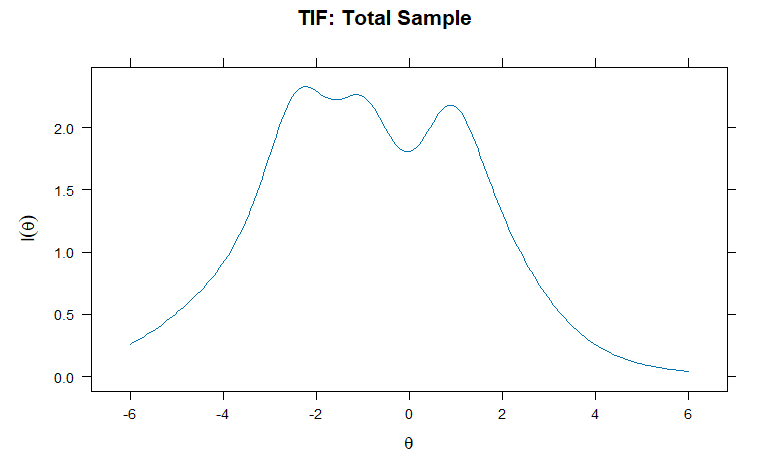
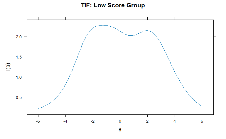
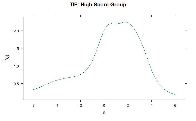
θ（潜在特性値）のテスト情報量をプロット

par(mfrow = c(3,1), mar = c(4,4,2,1))
plot(mod_total, type = "info", main = "TIF: Total Sample")
plot(mod_low,   type = "info", main = "TIF: Low Score Group")
plot(mod_high,  type = "info", main = "TIF: High Score Group")

ggplotを持つ板重ね書きプロット

# ライブラリ読み込み
library(ggplot2)
library(tidyr)

# θ のグリッドを作成
Theta <- matrix(seq(-4, 4, length = 201))

# 各モデルのテスト情報量を取得
info_total  <- testinfo(mod_total,  Theta)
info_low    <- testinfo(mod_low,    Theta)
info_high   <- testinfo(mod_high,   Theta)

# データフレームにまとめる
df <- data.frame(
  theta   = Theta[,1],
  Total   = info_total,
  Low     = info_low,
  High    = info_high
)

# 縦長フォーマットに変換
df_long <- pivot_longer(df, cols = -theta, 
                        names_to  = "Group", 
                        values_to = "Information")

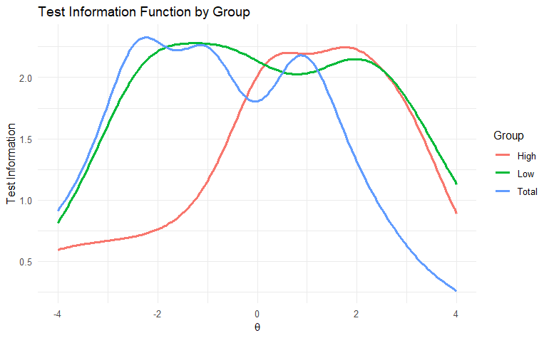
# ggplot2 で重ね描き
ggplot(df_long, aes(x = theta, y = Information, color = Group)) +
  geom_line(size = 1) +
  labs(
    x     = expression(theta),
    y     = "Test Information",
    title = "Test Information Function by Group"
  ) +
  theme_minimal()